DeepLagField

This tutorial demonstrates training a neural network to infer the order \(p\) and time-varying coefficients \(a(t)\) of TVAR processes:

\[x_t = \sum_{k=1}^{p} a_k(t) x_{t-k} + \varepsilon_t\]

Goals:

1. Generate synthetic TVAR data with known ground-truth coefficients

2. Train DeepLagField to jointly predict AR order and coefficient trajectories

3. Evaluate classification and regression accuracy across coefficient families

From a Waveform to a Local Dynamical Description

A waveform shows what a system did. A dynamical model describes how recent observations combine to produce its next value. For a time-varying autoregressive (TVAR) process, that relationship is allowed to change throughout an observation window:

\[x_t=\mathbf{a}_t^{\mathsf T}\mathbf{h}_t+\varepsilon_t, \qquad \mathbf{h}_t=[x_{t-1},\ldots,x_{t-p}]^{\mathsf T}.\]

Here \(\mathbf{h}_t\) is the observed lag history, \(\mathbf{a}_t\) contains the lag weights at time \(t\), and \(\varepsilon_t\) is the innovation not explained by that history. A conventional fixed-coefficient AR model estimates one vector for the entire window. DeepLagField instead estimates a coefficient trajectory together with the active AR order needed to represent the window.

The distinction matters when dynamics drift or change regime. Averaging over those changes can obscure which temporal relationships were present at a particular time. A time-indexed coefficient description can expose those changes, while order selection limits how many lags are active. The resulting coefficients are interpretable model parameters, rather than an unrestricted latent embedding.

In this implementation, one order is selected per input window; the coefficients vary within that window. Order is not independently selected at every time point. The neural estimator also receives the entire window, so coefficient inference is an offline window-level operation, not a causal streaming predictor.

Notation and Array Shapes

Symbol	Meaning	Setting used below
\(B\)	Number of sequences in a batch	Up to 256 during training
\(T\)	Samples per sequence	600
\(\mathcal P\)	Candidate AR orders	\(\{2,3,4,5,6\}\)
\(p_{\max}\)	Largest candidate order	6
\(\mathbf{x}\)	One observed sequence	Shape \((T,)\)
\(\widehat A\)	Estimated lag coefficients	Shape \((B,T,p_{\max})\)
\(\widehat p\)	Selected order per sequence	Shape \((B,)\)

Time indices in the synthetic schedules are samples, not seconds. A physical sampling rate is needed before assigning durations or Hz. The model’s order is a lag count, not automatically a count of oscillatory modes or a manifold dimension.

The cells below proceed from known synthetic dynamics to data preparation, joint inference, loss design, training, and three complementary evaluations: order selection, coefficient recovery, and waveform reconstruction. All existing figures are saved results; viewing this tutorial does not run training.

Show code

Hide code

import neuralfieldmanifold as nfm
import matplotlib.pyplot as plt
from pathlib import Path
import os
color_main, color_alt = "black", "darkred"
import torch
from torch.utils.data import DataLoader, TensorDataset
from sklearn.metrics import confusion_matrix, ConfusionMatrixDisplay
import numpy as np
from tqdm import tqdm
import matplotlib.pyplot as plt
import pandas as pd







from concurrent.futures import ProcessPoolExecutor, as_completed
import multiprocessing
from sklearn.model_selection import train_test_split

from matplotlib_inline.backend_inline import set_matplotlib_formats
set_matplotlib_formats("svg", "retina")

Coefficient Schedule Registry

Eight families control how \(a_k(t)\) evolve over time:

• sinusoid / fourier / quasiperiodic: Periodic or near-periodic oscillations

• poly_drift / logistic: Smooth trends and transitions

• multi_sigmoid / gaussian_bumps: Localized regime changes

• smooth_random: Stochastic but differentiable trajectories

What a Coefficient Schedule Controls

A schedule generates the hidden coefficients, not the signal directly. For example, a sinusoidal schedule can have the form

\[a_k(t)=c_k+A_k\sin(2\pi\nu_k t+\phi_k),\]

where \(c_k\) is a baseline lag weight, \(A_k\) its modulation amplitude, \(\nu_k\) its modulation rate, and \(\phi_k\) its phase. The observed waveform is then obtained by running the TVAR recursion with noise. A coefficient that varies sinusoidally does not imply that the waveform has a spectral peak at that same modulation frequency.

The registry spans several kinds of temporal organization. The expressions below summarize their construction; the actual generators vary parameters across lags and realizations.

Family	Schematic coefficient path	What it probes
sinusoid	\(c_k+A_k\sin(2\pi\nu_k t+\phi_k)\)	Smooth, repeating variation
fourier	\(c_k+\sum_m A_{km}\sin(2\pi m\nu_k t+\phi_{km})\)	Richer periodic shape
quasiperiodic	A sum of two differently paced oscillations	Multiple modulation timescales
poly_drift	\(c_k+\sum_d b_{kd}u^d\), with \(u\in[-1,1]\)	Gradual nonperiodic drift
logistic	\(a_{k,-}+(a_{k,+}-a_{k,-})s(t)\)	One smooth transition
multi_sigmoid	\(c_k+\sum_j\Delta_{kj}s_j(t)\)	Several transitions
gaussian_bumps	\(c_k+\sum_j A_{kj}e^{-(t-\mu_{kj})^2/(2w_{kj}^2)}\)	Localized excursions
smooth_random	Smoothed Gaussian noise around \(c_k\)	Smooth irregular variation

Here \(s(t)=[1+\exp(-(t-t_0)/w)]^{-1}\) is a logistic transition. The schedule family describes how coefficients change; the order \(p\) describes how many lag coefficients are available. The model predicts the order, not the family name. Grouping results by family later tests whether recovery changes with temporal pattern.

Show code

Hide code

# Registry of families you can benchmark
SCHEDULES = {
    "sinusoid": nfm.simulation.schedules.sinusoid,
    "fourier": nfm.simulation.schedules.fourier,
    "quasiperiodic": nfm.simulation.schedules.quasiperiodic,
    "poly_drift": nfm.simulation.schedules.polynomial_drift,
    "logistic": nfm.simulation.schedules.logistic_transition,
    "multi_sigmoid": nfm.simulation.schedules.multi_sigmoid,
    "gaussian_bumps": nfm.simulation.schedules.gaussian_bumps,
    "smooth_random": nfm.simulation.schedules.smooth_random,
}

Data Generation

Key functions:

• simulate_tvar(): Simulates TVAR with soft power clamping to prevent divergence

• generate_one_tvar_sample(): Produces a single \((x, a(t), \text{meta})\) tuple with retry logic

• generate_dataset(): Parallelized generation balanced across families and orders \(p \in \{2,...,6\}\)

Generate Signals with Known Coefficients and Controlled Scale

A training example consists of a waveform \(x_{0:T-1}\), a known coefficient path \(A\), and one generating order \(p\). Before any power correction, the simulator updates

\[u_t=\sum_{k=1}^{p}a_k(t)x_{t-k}+\varepsilon_t, \qquad \varepsilon_t\sim\mathcal N(0,\sigma^2).\]

The helper supplies 300 burn-in samples, using the first coefficient vector during that initial interval, and discards them before returning the requested waveform. This reduces dependence on initial history. A random seed controls coefficient generation and innovations so an accepted realization can be reproduced.

With power control enabled, the simulator computes rolling mean-square amplitude over \(W\) samples and applies a bounded correction to the current candidate sample:

\[P_t=\frac{1}{W}\left(u_t^2+\sum_{j=1}^{W-1}x_{t-j}^2\right),\qquad c_t=\operatorname{clip}\!\left(\sqrt{P_0/P_t},0.8,1.2\right), \qquad x_t=c_tu_t.\]

In this expression the current value is the candidate \(u_t\); the earlier values in its rolling history are the samples already stored by the simulation. The implementation applies the correction whenever rolling power is positive, not only when it exceeds the target. The defaults here are \(P_0=0.5\) and \(W=40\). Amplitude overflow or a final rolling-power violation rejects the realization, and the helper retries with another seed.

These steps define a controlled synthetic benchmark; they are not a proof of TVAR stability. Power correction is an additional operation beyond the unconstrained linear recursion, while the coefficient labels remain the supplied schedules. Keep that distinction in mind when interpreting recovery of the generating coefficients.

Store Different Orders in One Consistent Array

An order-\(p\) coefficient path is padded with zeros above lag \(p\):

\[\begin{split}A_{t,k}=\begin{cases}a_k(t),&k\leq p,\\0,&k>p.\end{cases}\end{split}\]

The dataset helper allocates 10 lag columns for storage. The network below supports orders only through 6, so evaluation later compares its output with A[:, :, :6]. Extra storage columns are not additional active model lags. Keeping signal, coefficients, order, and family aligned by example is essential when splitting and evaluating the data.

Show code

Hide code

def _rng(seed):
    return np.random.default_rng(seed)

def pad_to_pmax(a_time_p, p_max):
    """Pad [T, p_true] -> [T, p_max] with zeros."""
    T, p = a_time_p.shape
    out = np.zeros((T, p_max), dtype=a_time_p.dtype)
    out[:, :p] = a_time_p
    return out

def generate_one_tvar_sample(
    T=10_000,
    p_max=6,
    schedule_name="sinusoid",
    noise_std=0.3,
    seed=0,
    l1_cap=0.95,
    P0=0.5,
    W=40,
    power_control=True,
    p_true=None,  # If provided, use this p; otherwise random
    p_candidates=None,
    max_retries=10000,  # Maximum resampling attempts
):
    rng = _rng(seed)
    if p_candidates is None:
        p_candidates = np.array([2, 3, 4, 5, 6], dtype=int)
    
    # Use provided p_true or randomly select
    if p_true is None:
        p_true = int(rng.choice(p_candidates))
    else:
        p_true = int(p_true)

    # Retry loop: resample until we get a valid sample
    current_seed = seed
    for attempt in range(max_retries):
        # Use a fresh rng for coefficient schedule each attempt
        attempt_rng = _rng(current_seed)
        
        # coefficient schedule for true p
        a_tp = SCHEDULES[schedule_name](n_samples=T, order=p_true, rng=attempt_rng)

        # simulate signal with power control (rejection-based)
        x, a_actual = simulate_tvar(
            a_tp, noise_std=noise_std, seed=current_seed+123,
            P0=P0, W=W, power_control=power_control
        )

        # If valid sample (not rejected), break out
        if x is not None:
            break
        
        # Increment seed for next attempt
        current_seed += 1
    else:
        raise RuntimeError(f"Failed to generate valid sample after {max_retries} retries for schedule '{schedule_name}', p_true={p_true}")

    # pad coeffs to p_max for consistent storage
    a_t = pad_to_pmax(a_actual.astype(np.float32), p_max)

    meta = {
        "T": T,
        "p_max": p_max,
        "p_true": p_true,
        "schedule": schedule_name,
        "noise_std": float(noise_std),
        "seed": int(current_seed),  # Record the seed that actually worked
        "l1_cap": float(l1_cap),
        "P0": float(P0),
        "W": int(W),
        "power_control": power_control,
        "p_candidates": list(p_candidates),
        "retries": attempt,  # Number of retries needed
    }
    return x, a_t, meta

def _generate_sample_worker(args):
    """
    Worker function for parallel sample generation.
    Takes a dict of arguments and returns (idx, x, a_t, meta, cid, ns).
    """
    idx = args["idx"]
    T = args["T"]
    p_max = args["p_max"]
    cname = args["cname"]
    ns = args["ns"]
    s = args["s"]
    P0 = args["P0"]
    W = args["W"]
    power_control = args["power_control"]
    p_true_val = args["p_true_val"]
    p_candidates = args["p_candidates"]
    cid = args["cid"]
    
    x, a_t, meta = generate_one_tvar_sample(
        T=T, p_max=p_max, schedule_name=cname, noise_std=ns, seed=s,
        P0=P0, W=W, power_control=power_control,
        p_true=p_true_val, p_candidates=p_candidates,
    )
    
    return idx, x, a_t, meta, cid, ns

def simulate_tvar(a_time, noise_std=0.3, seed=0, burn_in=300,
                  P0=0.5, W=40, power_control=True,
                  divergence_threshold=1e6):
    """
    Simulate a TVAR process with soft power clamping and hard rejection safety net:
        x_t = a(t)^T [x_{t-1}, ..., x_{t-p}] + eps_t

    During simulation, if window power exceeds P0, the current sample is scaled
    by clip(sqrt(P0/power), 0.8, 1.2) to gently steer power back toward the target.
    After simulation, a final hard check rejects if power still exceeds P0.
    """
    try:
        x = nfm.simulation.tvar(
            a_time, noise_std=noise_std, seed=seed, burn_in_samples=burn_in,
            target_power=P0 if power_control else None, power_window_samples=W,
            max_abs=divergence_threshold,
        )
    except nfm.simulation.SimulationRejected:
        return None, None
    return x, a_time

def generate_dataset(
    n_per_class=10,
    classes=None,
    T=1000,
    noise_range=(0.1, 0.6),
    seed=0,
    dtype=np.float32,
    P0=0.5,
    W=40,
    power_control=True,
    p_candidates=None,
    balanced_p=True,  # If True, balance samples across p_candidates
    n_workers=None,  # Number of parallel workers (None = CPU count)
):
    
    p_max = 10
    
    if p_candidates is None:
        p_candidates = np.array([2, 3, 4, 5, 6], dtype=int)
    else:
        p_candidates = np.array(p_candidates, dtype=int)

    if classes is None:
        classes = list(SCHEDULES.keys())

    if n_workers is None:
        n_workers = multiprocessing.cpu_count()

    rng = _rng(seed)
    N = n_per_class * len(classes)

    X = np.zeros((N, T), dtype=dtype)
    A = np.zeros((N, T, p_max), dtype=dtype)
    p_true_arr = np.zeros((N,), dtype=np.int32)
    class_id = np.zeros((N,), dtype=np.int32)
    noise_std = np.zeros((N,), dtype=dtype)

    class_names = list(classes)
    
    # Precompute p assignments if balanced
    n_p = len(p_candidates)
    if balanced_p:
        n_per_p = n_per_class // n_p
        remainder = n_per_class % n_p
        # Create balanced p assignments for one class
        p_assignments = []
        for i, p in enumerate(p_candidates):
            count = n_per_p + (1 if i < remainder else 0)
            p_assignments.extend([p] * count)
    
    # Build all task arguments
    tasks = []
    idx = 0
    for cid, cname in enumerate(class_names):
        # Shuffle p assignments for this class
        if balanced_p:
            class_p_assignments = rng.permutation(p_assignments)
        
        for i in range(n_per_class):
            s = int(rng.integers(0, 2**31 - 1))
            ns = float(rng.uniform(noise_range[0], noise_range[1]))
            
            # Determine p_true
            if balanced_p:
                p_true_val = int(class_p_assignments[i])
            else:
                p_true_val = None  # Let generate_one_tvar_sample pick randomly
            
            tasks.append({
                "idx": idx,
                "T": T,
                "p_max": p_max,
                "cname": cname,
                "ns": ns,
                "s": s,
                "P0": P0,
                "W": W,
                "power_control": power_control,
                "p_true_val": p_true_val,
                "p_candidates": list(p_candidates),
                "cid": cid,
            })
            idx += 1
    
    metas = [None] * N
    
    # Parallel execution
    with ProcessPoolExecutor(max_workers=n_workers) as executor:
        futures = {executor.submit(_generate_sample_worker, task): task["idx"] for task in tasks}
        
        with tqdm(total=N, desc=f"Generating samples ({n_workers} workers)") as pbar:
            for future in as_completed(futures):
                idx, x, a_t, meta, cid, ns = future.result()
                X[idx] = x.astype(dtype)
                A[idx] = a_t.astype(dtype)
                p_true_arr[idx] = meta["p_true"]
                class_id[idx] = cid
                noise_std[idx] = ns
                metas[idx] = meta
                pbar.update(1)

    dataset = {
        "X": X,
        "A": A,
        "p_true": p_true_arr,
        "class_id": class_id,
        "class_names": np.array(class_names),
        "noise_std": noise_std,
        "meta": metas,  # Python list of dicts; fine for notebook use
    }
    return dataset

def save_dataset_npz(path, dataset):
    np.savez(
        path,
        X=dataset["X"],
        A=dataset["A"],
        p_true=dataset["p_true"],
        class_id=dataset["class_id"],
        class_names=dataset["class_names"],
        noise_std=dataset["noise_std"],
        meta=np.array(dataset["meta"], dtype=object),
    )

def load_dataset_npz(path):
    d = np.load(path, allow_pickle=True)
    return {
        "X": d["X"],
        "A": d["A"],
        "p_true": d["p_true"],
        "class_id": d["class_id"],
        "class_names": d["class_names"],
        "noise_std": d["noise_std"],
        "meta": list(d["meta"]),
    }

Visualize Schedule Families

Each schedule produces qualitatively different signals. Top row shows \(x(t)\); bottom row shows the true \(a_k(t)\) coefficients. Note how coefficient dynamics translate into signal structure.

Read the Signal and Coefficient Panels Together

Each column displays one independently generated example of a schedule family. The upper panel is the noisy waveform; the lower panel shows the actual active lag weights. The example order is drawn from the candidate set, so different columns need not have the same number of coefficient curves.

Look first for the lower panel’s organizing pattern: repetition, drift, a transition, or a localized event. Then ask whether its effect is recognizable in the waveform. The mapping is indirect because each value combines lagged observations and a new innovation. A visually noisy waveform can still arise from a smooth coefficient path, and similar-looking waveforms can arise from different paths.

This is why the later benchmark checks coefficients as well as reconstruction error. The gallery is a guide to the families, not a trained model’s output or an estimate of its accuracy. The gallery chooses fresh random seeds when executed, so rerunning this cell can change the individual examples.

Show code

Hide code

# Plot one example of each schedule type: signal (top row) + coefficients (bottom row)
schedule_names = list(SCHEDULES.keys())

fig, axes = plt.subplots(2, 8, figsize=(24, 6))

for i, schedule_name in enumerate(schedule_names):
    x, a_t, meta = generate_one_tvar_sample(
        T=600, p_max=10,
        schedule_name=schedule_name,
        noise_std=0.3,
        seed=np.random.randint(0, 2**31 - 1)
    )
    
    p_true = meta["p_true"]
    
    # Top row: signal
    ax_sig = axes[0, i]
    ax_sig.plot(x, alpha=0.7, linewidth=0.5)
    ax_sig.set_title(schedule_name, fontsize=10)
    ax_sig.grid(True, alpha=0.3)
    if i == 0:
        ax_sig.set_ylabel("x(t)")
    
    # Bottom row: coefficients
    ax_coef = axes[1, i]
    for k in range(p_true):
        ax_coef.plot(a_t[:, k], label=f"a{k+1}(t)", alpha=0.8)
    ax_coef.grid(True, alpha=0.3)
    if i == 0:
        ax_coef.set_ylabel("Coefficient value")
    ax_coef.set_xlabel("t")

plt.tight_layout()
plt.show()

Generate Training Dataset

Create a balanced dataset: equal samples per family, uniform distribution over \(p \in \{2,3,4,5,6\}\), and noise \(\sigma \in [0.2, 0.5]\). Power control ensures bounded variance.

Balance the Generating Conditions

The pilot call requests 10 examples per family, eight families, and 600 samples per waveform: 80 examples in total. Each family receives two examples of every order in \(\{2,3,4,5,6\}\). The assigned orders are shuffled within the family, and the innovation standard deviation is drawn from \([0.2,0.5]\).

Balancing avoids teaching order selection mainly from the most common category and makes family-specific comparisons more interpretable. Varying noise makes the task broader than identifying one clean coefficient trajectory. The accepted signal distribution also depends on the simulation’s power control and rejection steps described above.

The returned arrays have shapes

\[X\in\mathbb R^{N\times600},\qquad A\in\mathbb R^{N\times600\times10},\qquad p_{\mathrm{true}},\;\mathrm{class\_id}\in\mathbb Z^N.\]

class_id identifies the schedule family for later grouping; it is not the target label for the order classifier. This small pilot illustrates dataset construction. The following cell loads a saved dataset for the benchmark; it does not automatically train on pilot.

Show code

Hide code

classes = list(SCHEDULES.keys())

# small pilot: 10 per family => 80 samples total
pilot = generate_dataset(
    n_per_class=10, 
    classes=classes,
    T=600,
    noise_range=(0.2, 0.5),
    seed=123,
    dtype=np.float32
)
# save_dataset_npz("train_data.npz", pilot)

Load the Benchmark and Split Whole Examples

Set NFM_TVAR_DATA_FILE to the saved .npz file, or place train_data.npz in the notebook’s working directory. The loader reads waveform, coefficient, order, and family arrays from that file. Saving the pilot is shown in the preceding cell but is commented out; creating the pilot alone does not create the file being loaded here.

The split assigns 80% of complete sequences to training and 20% to validation, stratified by generating AR order, with random_state=42. It does not split each 600-sample sequence into an early training interval and a later validation interval. Every coefficient path follows the same example indices as its waveform.

This evaluates recovery on other examples from the supplied dataset. Stratification explicitly preserves order proportions, not necessarily exact family-by-order counts. The family and order summaries therefore complement each other. This is not a held-out-family experiment: the same schedule families can appear on both sides of the split. The actual dataset size is printed by the loader rather than inferred from the separate pilot-generation settings.

Show code

Hide code

benchmark_path = Path(os.environ.get("NFM_TVAR_DATA_FILE", "train_data.npz"))
with np.load(benchmark_path, allow_pickle=False) as data:
    X_all, coefficients_all = data["X"], data["A"]
    orders_all, families_all = data["p_true"], data["class_id"]
    class_names = data["class_names"]
train_indices, validation_indices = train_test_split(
    np.arange(len(X_all)), train_size=0.8, stratify=orders_all, random_state=42
)
X_train, X_val = X_all[train_indices], X_all[validation_indices]
coef_train, coef_val = coefficients_all[train_indices], coefficients_all[validation_indices]
p_train, p_val = orders_all[train_indices], orders_all[validation_indices]
class_id_train, class_id_val = families_all[train_indices], families_all[validation_indices]
print(f"Total samples: {len(X_all)} | Train: {len(X_train)} | Val: {len(X_val)}")
print(f"Train p distribution: {dict(zip(*np.unique(p_train, return_counts=True)))}")
print(f"Val p distribution:   {dict(zip(*np.unique(p_val, return_counts=True)))}")

Total samples: 1000000 | Train: 800000 | Val: 200000
Train p distribution: {np.int64(0): np.int64(160000), np.int64(1): np.int64(160000), np.int64(2): np.int64(160000), np.int64(3): np.int64(160000), np.int64(4): np.int64(160000)}
Val p distribution:   {np.int64(0): np.int64(40000), np.int64(1): np.int64(40000), np.int64(2): np.int64(40000), np.int64(3): np.int64(40000), np.int64(4): np.int64(40000)}

Prepare DataLoaders

Move tensors to GPU upfront to eliminate per-batch transfer overhead. The model expects shape (batch, T) for signals and (batch,) for order labels.

Separate Training Inputs from Evaluation Ground Truth

A batch supplies

\[X_{\mathrm{batch}}\in\mathbb R^{B\times600},\qquad p_{\mathrm{batch}}\in\{2,3,4,5,6\}^{B}.\]

Signals are floating-point tensors; order labels are integer tensors containing the actual AR orders, not zero-based class indices. Batches contain up to 256 examples. Shuffling changes the order in which whole sequences are presented, not the temporal order within a waveform.

Importantly, the TensorDataset contains signals and orders only. The known coefficient arrays are retained for later evaluation and are not passed to the training loss. Coefficient recovery is therefore learned through signal reconstruction and regularization, with supervised order selection, rather than direct coefficient-target regression in this training call.

The cell chooses an available CUDA device, preferring the second GPU when present, and otherwise uses CPU. This affects where computation runs, not the mathematical meaning of a sequence or order label.

Show code

Hide code

device = torch.device(('cuda:1' if torch.cuda.device_count() > 1 else 'cuda:0') if torch.cuda.is_available() else 'cpu')
if device.type == 'cuda':
    torch.cuda.init()
    torch.backends.cudnn.benchmark = True
    print(f"Using device: {device}")

# Move ALL data to GPU upfront - eliminates CPU->GPU transfer bottleneck
X_train = torch.tensor(X_train, dtype=torch.float32, device=device)
p_train = torch.tensor(p_train, dtype=torch.long, device=device)
X_val = torch.tensor(X_val, dtype=torch.float32, device=device)
p_val = torch.tensor(p_val, dtype=torch.long, device=device)
class_id_val = class_id_val  # numpy array

# Data already on GPU - no pin_memory/workers needed
train_loader = DataLoader(
    TensorDataset(X_train, p_train), 
    batch_size=256,
    shuffle=True
)
val_loader = DataLoader(
    TensorDataset(X_val, p_val), 
    batch_size=256
)

Using device: cuda:1

Define Training Configuration

Loss function combines:

• lambda_p: Cross-entropy for order classification

• lambda_ar: MSE between predicted and true coefficients

• lambda_energy: Penalizes large coefficient magnitudes within the prediction window

• lambda_smooth: Encourages temporally smooth \(\hat{a}(t)\)

Architecture: An Order Network and a Dynamics Network

DeepLagField combines a discrete structural choice with continuous coefficient estimation. The order network maps the complete waveform to one logit per candidate order:

\[\boldsymbol\ell=f_{\mathrm{order}}(\mathbf{x})\in\mathbb R^5, \qquad q_j=\frac{e^{\ell_j}}{\sum_{r=0}^{4}e^{\ell_r}},\quad p_j\in(2,3,4,5,6).\]

A logit is an unnormalized category score; \(q_j\) is its softmax probability. These are scores for different lag counts, not probabilities that particular time points are oscillatory.

The dynamics network receives the waveform concatenated with the selected-order indicator \(\mathbf{s}\) and outputs a coefficient value for every time and candidate lag:

\[\widetilde A=\operatorname{reshape} \left(f_{\mathrm{dyn}}([\mathbf{x};\mathbf{s}]),\;T,p_{\max}\right).\]

Both networks are multilayer perceptrons with two hidden layers of width 128 and ReLU activations. With \(T=600\), the order network maps \(600\to128\to128\to5\), while the dynamics network maps \(605\to128\to128\to3600\). The latter’s 3,600 outputs are reshaped into \(600\times6\) coefficients.

A single network pass thus estimates an entire coefficient field across a fixed-length window. It is not a recurrent update that sees only the samples available before each output time, and the coefficient estimates may use context from anywhere in the input window.

Train through a Discrete Order Choice

Taking an argmax gives a clear category but does not supply ordinary derivatives through that choice. During training, the order block uses hard straight-through Gumbel-softmax sampling. Conceptually, draw \(u_j\sim\mathrm{Uniform}(0,1)\) and form

\[g_j=-\log(-\log u_j),\qquad s_j^{\mathrm{soft}}= \frac{\exp((\ell_j+g_j)/\theta)} {\sum_r\exp((\ell_r+g_r)/\theta)}.\]

The temperature \(\theta>0\) controls the sharpness of the soft selection. The forward pass uses a one-hot vector at its largest entry; the backward pass uses the soft selection’s derivatives:

\[\mathbf{s}_{\mathrm{ST}}= \operatorname{stopgrad} (\mathbf{s}_{\mathrm{hard}}-\mathbf{s}_{\mathrm{soft}}) +\mathbf{s}_{\mathrm{soft}}.\]

This lets the dynamics network operate with one selected order while providing a gradient through its order-conditioning input. It is a gradient estimator, not exact differentiation through an integer. The lag-support mask described next is applied using the hard order; it is not a continuously valued mask in the forward computation.

The training configuration uses the default temperature 1.0. Ordinary evaluation uses the largest logit without sampling unless sample_order=True is requested. Several evaluation cells below explicitly request sampling, a distinction relevant when comparing repeated runs of their metrics.

Enforce the Chosen Lag Support and Reconstruct the Signal

The selected order determines which lag columns are permitted:

\[m_k(\widehat p)=\mathbf{1}\{k\leq\widehat p\},\qquad \widehat a_k(t)=m_k(\widehat p)\widetilde a_k(t).\]

For example, selecting order 3 makes columns 4-6 exactly zero at every time, while columns 1-3 may change within the window. Active columns are allowed to be small or zero; the selected order is the supported lag count, not a guarantee that each active weight is large.

The model reconstructs the input using those coefficients and observed lagged samples:

\[\widehat x_t=\sum_{k=1}^{p_{\max}} \widehat a_k(t)x_{t-k}.\]

There is no separate intercept in this neural reconstruction. Missing history at the window start is zero-padded, and reconstruction MSE excludes the first \(p_{\max}=6\) samples. For a batch, the output contains coefficient shape \((B,600,6)\), logits shape \((B,5)\), selected orders shape \((B,)\), and predictions shape \((B,600)\).

Because the coefficients are inferred from the full window and the reconstruction uses observed history, this is a window-conditioned dynamical reconstruction, not a held-out future forecast or an autonomous simulation. The supervision and regularizers below make that reconstruction problem more constrained than unconstrained waveform fitting.

The Training Objective and Its Exact Loss Names

The executable configuration below combines five terms:

\[\mathcal L= \lambda_{\mathrm{ar}}\mathcal L_{\mathrm{rec}} +\lambda_p\mathcal L_{\mathrm{cls}} +\lambda_{\mathrm{energy}}\mathcal L_{\mathrm{power}} +\lambda_{\mathrm{smooth}}\mathcal L_{\mathrm{smooth}} +\lambda_{\mathrm{order}}\mathcal L_{\mathrm{size}}.\]

For this call, lambda_ar weights signal reconstruction MSE, not MSE against the known coefficient paths. Likewise, lambda_energy weights predicted waveform power, not coefficient magnitude. The explicit definitions below specify the objective used by nfm.training.compute_losses; coefficient MSE appears later as an evaluation metric.

Each term addresses a different ambiguity. Reconstruction asks the coefficients to explain the observed waveform. Classification teaches which lag support is appropriate. Power constrains amplitude scale, and smoothness discourages coefficients from changing arbitrarily between neighboring samples. The optional size penalty favors smaller candidate-order indices but is disabled in this example.

Signal Reconstruction: Explain the Observed Local Evolution

For a batch of \(B\) windows, the reconstruction term is

\[\mathcal L_{\mathrm{rec}}= \frac{1}{B(T-p_{\max})} \sum_{b=1}^{B}\sum_{t=p_{\max}}^{T-1} \left(x_{b,t}-\sum_{k=1}^{p_{\max}} \widehat a_{b,k}(t)x_{b,t-k}\right)^2.\]

Time is indexed from zero, whereas lag \(k\) starts at 1. Excluding the leading maximum-order context gives every candidate order a common interval with complete lag history. The term rewards the estimated dynamics for accounting for the signal rather than merely producing plausible-looking coefficient curves.

It cannot by itself identify a unique coefficient vector at every time. There is one scalar reconstruction equation and potentially several unknown coefficients. Noise and correlated lag histories create further ambiguity. Accurate waveform reconstruction must therefore be considered alongside coefficient recovery and the constraints imposed by the other losses.

The dynamical constraint is built into the reconstruction itself: the predicted waveform must be assembled from inferred coefficients and lagged observations, rather than emitted by an unrelated waveform decoder. This is the physics-informed aspect of the estimator here. It imposes the chosen autoregressive structure, not a universal conservation law or an automatic guarantee of a particular manifold.

Order Classification: Learn the Structural Choice

Let \(c(p_b)\) be the index of example \(b\)’s true order in the candidate list. Cross-entropy gives

\[\mathcal L_{\mathrm{cls}}= -\frac{1}{B}\sum_{b=1}^{B}\log q_{b,c(p_b)}.\]

With candidates \((2,3,4,5,6)\), the corresponding internal class indices are \((0,1,2,3,4)\), but the public training labels remain the actual orders. The loss converts them to candidate positions before evaluating cross-entropy.

This term teaches order directly from the synthetic generating labels. Reconstruction alone could often be improved using extra lags, so a small waveform error would not necessarily teach the desired order. Cross-entropy uses the order logits, while the selected order also conditions the dynamics network and fixes its available lag support. The two tasks are coupled, but they are not the same target.

Predicted Power: Constrain the Waveform’s Amplitude Scale

The energy term compares rolling mean-square prediction amplitude with a fixed target. With \(W=40\), define windows beginning after the first \(W\) predicted samples:

\[\widehat P_{b,s}=\frac{1}{W}\sum_{j=0}^{W-1} \widehat x_{b,s+j}^{\,2},\qquad s=W,\ldots,T-W.\]

The loss is

\[\mathcal L_{\mathrm{power}}= \frac{1}{B(T-2W+1)}\sum_{b=1}^{B}\sum_{s=W}^{T-W} (\widehat P_{b,s}-P_0)^2,\qquad P_0=0.5.\]

This discourages predictions with a rolling amplitude scale far from the chosen synthetic target, complementing samplewise reconstruction. It uses the same numerical target and window length as the generation defaults, but it is a training penalty, not the simulator’s multiplicative power correction or rejection rule.

Mean square is not mean-subtracted variance, and the loss is not an \(L^2\) penalty on the coefficients. It does not constrain spectral peaks, oscillation frequencies, or topology. When applying the method to data on another amplitude scale, the target power and its weight must be chosen with that scale in mind.

Smoothness: Prefer Coherent Coefficient Trajectories

The coefficient-smoothness term penalizes first differences:

\[\mathcal L_{\mathrm{smooth}}= \frac{1}{B(T-1)}\sum_{b=1}^{B}\sum_{t=0}^{T-2} \sum_{k=1}^{p_{\max}} \left(\widehat a_{b,k}(t+1)-\widehat a_{b,k}(t)\right)^2.\]

It sums over lag columns and averages over examples and neighboring time pairs. The intended prior is that a local dynamical description should usually evolve coherently rather than using a different, unrelated coefficient vector for every sample. Constant paths have zero smoothness cost; smooth nonconstant paths remain possible when the reconstruction term supports them.

Stronger smoothing can suppress samplewise jitter but can also flatten transitions, reduce excursion amplitude, or lag a changing coefficient pattern. This trade-off is especially visible when comparing smooth drift with localized bumps or multiple transitions. The loss is in sample-index differences, not a physical derivative divided by a sampling interval, so changing temporal resolution changes its effective interpretation.

The optional size term uses the expected candidate index:

\[\mathcal L_{\mathrm{size}}= \frac{1}{B}\sum_{b=1}^{B}\sum_{j=0}^{4}j\,q_{b,j}.\]

For this ordered candidate set, larger indices mean larger AR orders. lambda_order=0 makes this term contribute nothing to the objective; no nonzero size preference should be attributed to this configuration.

Show code

Hide code

def do_bench_on_config(lambda_config, model=None):
    n_epochs = 100
    lr = 1e-3
    max_ar_order = 6
    if model is None:
        model = nfm.models.DeepLagField(sequence_length=600, orders=(2, 3, 4, 5, 6), hidden_size=128).to(device)
    weights = nfm.training.LossWeights(
        reconstruction=lambda_config["lambda_ar"],
        order_classification=lambda_config["lambda_p"],
        energy=lambda_config["lambda_energy"],
        smoothness=lambda_config["lambda_smooth"],
        order_penalty=lambda_config["lambda_order"],
    )
    config = nfm.training.TrainingConfig(
        epochs=n_epochs, learning_rate=lr, weights=weights,
        stochastic_validation=True,
    )
    history = nfm.training.train(model, train_loader, validation_loader=val_loader, config=config, device=device)
    return model, history

Train Model

Train for 100 epochs with balanced loss weights. The training curve shows joint convergence of classification and regression objectives.

Read the Weights as Trade-offs, Not Comparable Error Units

The configuration assigns

\[\mathcal L=5\mathcal L_{\mathrm{rec}} +5\mathcal L_{\mathrm{cls}} +0.2\mathcal L_{\mathrm{power}} +5\mathcal L_{\mathrm{smooth}}.\]

Equal numerical weights do not imply equal influence. Cross-entropy, waveform squared error, squared power error, and coefficient differences have different natural scales and different gradients. For example, multiplying the input amplitude changes the reconstruction and power terms in different ways, even if the coefficient paths are unchanged. The separate loss panels help identify which part of the objective is changing, rather than relying only on the total.

The model trains for 100 epochs, with batch size 256 and Adam learning rate \(10^{-3}\). The package clips the parameter-gradient norm to 1.0 and uses ReduceLROnPlateau with patience 10 and factor 0.5, monitoring validation total loss when available. Those are optimization choices, distinct from temporal smoothing of the inferred coefficients.

stochastic_validation=True means validation also samples orders. Validation does not update model parameters, but the sampled choices can add variability to its losses and accuracy. The configuration does not average multiple order samples for each validation example.

Show code

Hide code

conf = {
    "lambda_ar": 5,
    "lambda_p": 5,
    "lambda_order": 0,
    "lambda_energy": 0.2,
    "lambda_smooth": 5,
}

model, history = do_bench_on_config(conf)
nfm.plotting.training_history(history, model=model, validation_loader=val_loader, device=device)
plt.show()

Training: 100%|██████████| 100/100 [14:56<00:00,  8.96s/it, p_acc=0.340, train=6.5934, val=8.4380]

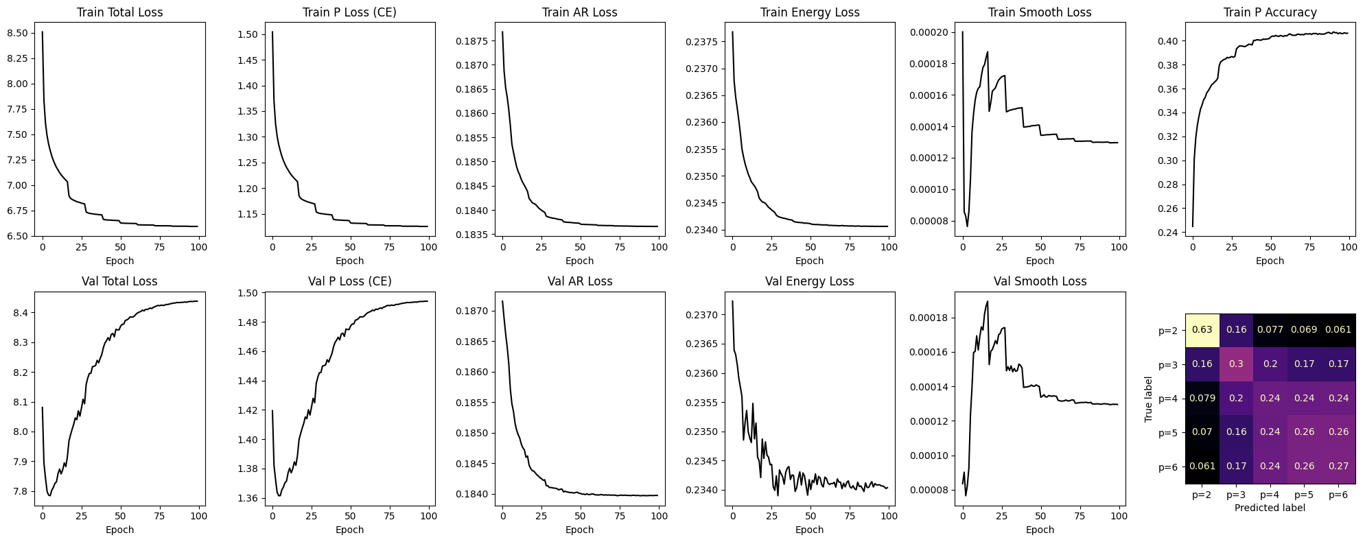
Interpret the Training Dashboard

The figure separates total loss, order cross-entropy, reconstruction, power, smoothness, and order accuracy. The individual loss panels show the component values before multiplying by their configured weights; total loss is their weighted combination. A component can rise while the total falls if improvements elsewhere outweigh it.

Read training and validation together. Falling training error alone does not establish recovery on other sequences. A widening gap can indicate specialization to the training examples, while fluctuating validation values can partly reflect sampled order choices. The curves are records of this optimization run, not confidence intervals across independent training runs.

The final validation panel is an aggregate order confusion matrix rather than a coefficient-error curve. Coefficient recovery is evaluated separately below because low reconstruction error and correct order are useful but not sufficient evidence of the correct time-varying lag weights.

Evaluation: Order Classification

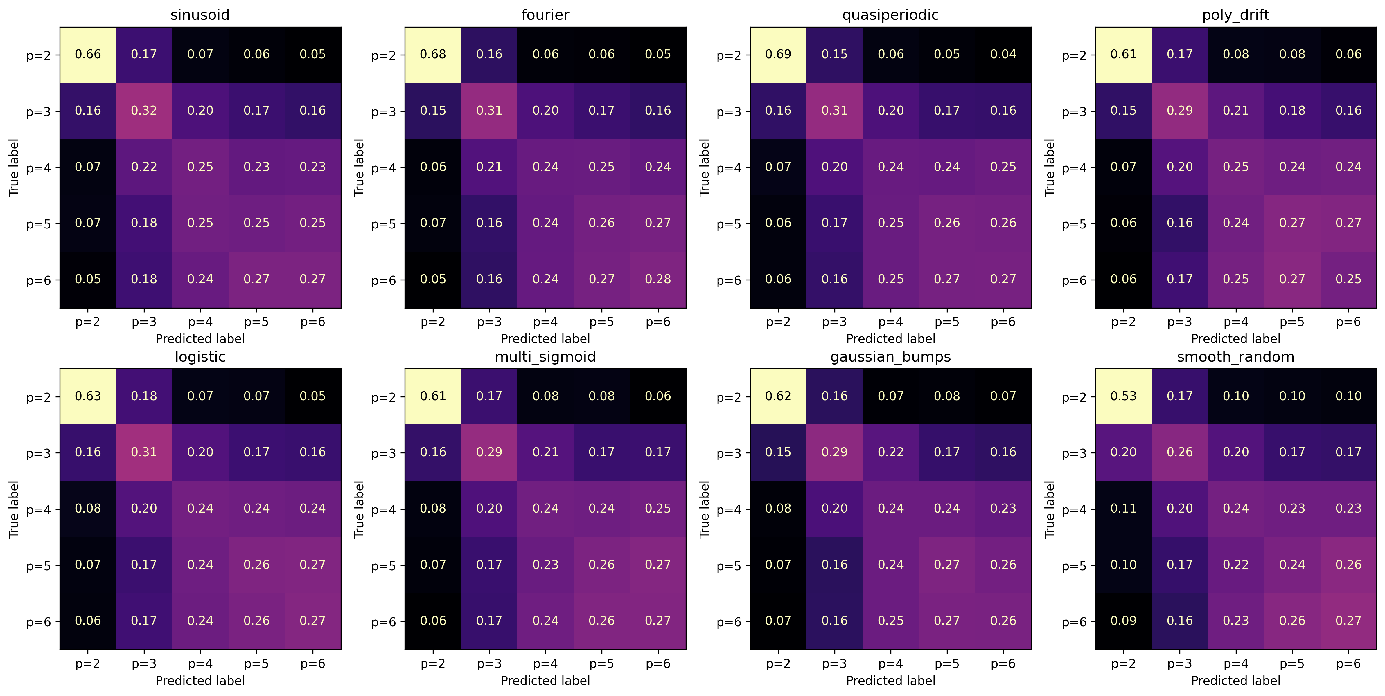
Confusion matrices show how well the model distinguishes AR orders within each family. Diagonal dominance indicates correct classification; off-diagonal mass reveals systematic over/under-estimation of \(p\).

Decide Which Order-Selection Protocol Is Being Evaluated

Calling model.eval() selects evaluation behavior, but the next cell additionally passes sample_order=True. It therefore draws an order through Gumbel sampling instead of always taking

\[\widehat p=p_{\operatorname{argmax}_j\ell_j}.\]

One sampled order is collected per validation example. A second evaluation can yield different assignments, even for the same weights and waveforms, when the random state changes. The family benchmark and coefficient-plot helpers also request their own sampled choices, so they need not reuse the exact decisions in this first pass.

For deterministic inference, model(x, sample_order=False) or the default call on an evaluation-mode model uses the largest logit. This describes an alternative protocol; it does not change the saved sampled-order results shown in the following cells. Keep the protocol fixed when comparing models or reported metrics.

Show code

Hide code

# Get predictions on full validation set
model.eval()
all_p_pred = []
all_p_true = []

with torch.no_grad():
    for x_batch, p_batch in tqdm(val_loader, desc="Getting predictions"):
        x_batch = x_batch.to(device)
        p_hard = model(x_batch, sample_order=True).order
        all_p_pred.extend(p_hard.cpu().numpy())
        all_p_true.extend(p_batch.cpu().numpy())

all_p_pred = np.array(all_p_pred)
all_p_true = np.array(all_p_true)

Getting predictions: 100%|██████████| 782/782 [00:00<00:00, 795.68it/s]

Read a Family-Specific Confusion Matrix

For family \(f\), let \(C^{(f)}_{ij}\) count examples whose true order is \(p_i\) and whose selected order is \(p_j\). The displayed entries are normalized within each true-order row:

\[\widetilde C^{(f)}_{ij}= \frac{C^{(f)}_{ij}}{\sum_r C^{(f)}_{ir}}.\]

A diagonal entry is the fraction of that true-order group classified correctly. Entries to its right indicate larger predicted orders; entries to its left indicate smaller predicted orders. Each row with observations sums to 1, regardless of how many examples it contains. These fractions are not uncertainty intervals.

Comparing families asks whether the same order is easier to recover under periodic variation, drift, or transitions. The model is not being asked to classify the eight families. A well-performing family should be assessed across its order rows, rather than by one visually strong diagonal cell. Families with different validation counts can have differently reliable fractions even when their colors match.

Show code

Hide code

# Plot confusion matrix for each signal family
n_families = len(class_names)
nrows, ncols = 2, 4
fig, axes = plt.subplots(nrows, ncols, figsize=(4 * ncols, 4 * nrows), dpi=300)
axes_flat = axes.flatten()

p_min, p_max = 2, 6
n_classes = p_max - p_min + 1

family_results = {}

for i, family_name in enumerate(class_names):
    mask = class_id_val == i
    p_true_family = all_p_true[mask]
    p_pred_family = all_p_pred[mask]
    
    # Compute normalized confusion matrix
    cm = confusion_matrix(p_true_family, p_pred_family, labels=range(p_min, p_max + 1))
    cm_norm = cm / cm.sum(axis=1, keepdims=True)
    
    # Store accuracy for this family
    family_results[family_name] = {
        'accuracy': np.mean(p_true_family == p_pred_family),
        'n_samples': len(p_true_family)
    }
    
    # Plot
    disp = ConfusionMatrixDisplay(cm_norm, display_labels=[f'p={j+p_min}' for j in range(n_classes)])
    disp.plot(ax=axes_flat[i], cmap='magma', colorbar=False, values_format='.2f')
    axes_flat[i].set_title(f'{family_name}')

# Hide unused subplots
for j in range(n_families, nrows * ncols):
    axes_flat[j].set_visible(False)

plt.tight_layout()
plt.show()

Benchmark: Coefficient Recovery

Metrics per family:

• coeff_mse: Mean squared error of \(\hat{a}(t)\) vs true \(a(t)\)

• signal_mse: One-step prediction error using estimated coefficients

• p_acc: Classification accuracy for each order

Evaluate Structure, Parameters, and Reconstruction Separately

The family benchmark reports three kinds of performance. For \(N\) sequences in a family, coefficient error is

\[\mathrm{MSE}_{a}=\frac{1}{NTp_{\max}} \sum_{n,t,k}\left(\widehat a_{n,k}(t)-a_{n,k}(t)\right)^2.\]

This includes all time positions and all six output lag columns, including zero-padded inactive coefficients. If the order is underestimated, a genuinely active coefficient can be masked to zero. If it is overestimated, extra nonzero lag weights can also increase error. It is therefore a joint measure of lag-support and coefficient recovery, not error restricted only to correctly selected active lags.

Signal error is

\[\mathrm{MSE}_{x}=\frac{1}{N(T-p_{\max})} \sum_n\sum_{t=p_{\max}}^{T-1} (\widehat x_{n,t}-x_{n,t})^2.\]

As in training, this uses observed lag history and window-conditioned coefficients, excluding the leading six samples. It is not an autonomous forecast score. Ground-truth coefficients enter the evaluation comparison, not this model’s training batches.

The order summaries use \(\Delta p_n=\widehat p_n-p_n\):

\[\begin{split}\begin{aligned} \mathrm{accuracy}_p&=N^{-1}\sum_n\mathbf 1\{\Delta p_n=0\},\\ \mathrm{MAE}_p&=N^{-1}\sum_n|\Delta p_n|,\\ \mathrm{relative\ error}_p&=N^{-1}\sum_n|\Delta p_n|/p_n,\\ \mathrm{accuracy}_{\leq1}&=N^{-1}\sum_n\mathbf 1\{|\Delta p_n|\leq1\}. \end{aligned}\end{split}\]

Exact accuracy treats every wrong order as incorrect; MAE distinguishes a one-lag miss from a larger error. Relative error divides by the true order and is returned as a fraction, not multiplied by 100. Per-order accuracies condition on one generating order within a family, while p_acc averages over all examples of that family.

Why a Good Reconstruction May Still Have Wrong Coefficients

At one time point, several coefficient vectors can produce almost the same scalar prediction. If a perturbation satisfies

\[\Delta\mathbf a_t^{\mathsf T}\mathbf h_t\approx0,\]

then \(\widehat{\mathbf a}_t\) and \(\widehat{\mathbf a}_t+\Delta\mathbf a_t\) reconstruct nearly the same value from that history. Strongly correlated lagged samples make such ambiguity especially relevant. Smoothness and training across many sequences reduce flexibility, but do not make every coefficient path uniquely identifiable from one noisy waveform.

This motivates reading the benchmark columns together. Low signal MSE with larger coefficient MSE means the inferred rule reproduces observations better than it reproduces the known generating weights. Correct order with poor trajectory tracking means the structural decision is easier than the parameter inference. Good coefficient MSE averaged over all columns can also conceal a localized error, motivating the overlays below.

The table summarizes performance on the supplied validation sequences. It does not by itself measure uncertainty over training seeds, generalization to unseen schedule families, or recovery in a new recording modality.

Show code

Hide code

family_bench_results = {}

for i, family_name in enumerate(class_names):
    mask = class_id_val == i
    X_family = X_val[mask].cpu()  # Move to CPU for bench_loop
    coef_family = coef_val[mask][:, :, :6]  # Slice to max_ar_order=6
    p_family = p_val[mask].cpu()
    
    evaluation = nfm.training.evaluate(
        model, X_family, true_coefficients=coef_family, true_orders=p_family.numpy(),
        device=device, sample_order=True,
    )
    actual = p_family.numpy()
    results = {
        "coeff_mse": evaluation["coefficient_mse"],
        "signal_mse": evaluation["prediction_mse"],
        "p_mae": evaluation["order_mae"],
        "p_mape": evaluation["order_relative_error"],
        "p_acc": evaluation["order_accuracy"],
        "p_acc_one": evaluation["within_one_accuracy"],
    }
    for order in model.orders:
        selected = actual == order
        results[f"p{order}_acc"] = float(np.mean(evaluation["order"][selected] == actual[selected])) if selected.any() else 0.0
    family_bench_results[family_name] = results

# Display as DataFrame
family_bench_df = pd.DataFrame(family_bench_results).T
family_df = family_bench_df.rename(columns={
    'coeff_mse': 'coeff mse',
    'signal_mse': 'signal mse',
    'p_mae': 'delta p',
    'p_mape': 'delta p / p',
    'p2_acc': 'p=2',
    'p3_acc': 'p=3',
    'p4_acc': 'p=4',
    'p5_acc': 'p=5',
    'p6_acc': 'p=6',
    'p_acc': 'P Avg.',
})
family_bench_df

	coeff_mse	signal_mse	p_mae	p_mape	p2_acc	p3_acc	p4_acc	p5_acc	p6_acc	p_acc
sinusoid	0.003924	0.183046	1.085483	0.290002	0.661209	0.326721	0.241122	0.251023	0.267625	0.351111
fourier	0.004272	0.184083	1.069846	0.284058	0.679984	0.316788	0.244737	0.274840	0.280372	0.358101
quasiperiodic	0.004035	0.182153	1.063116	0.281938	0.684039	0.310689	0.247123	0.272243	0.277012	0.356821
poly_drift	0.004315	0.183816	1.109580	0.302322	0.618354	0.300617	0.248848	0.262569	0.266481	0.340402
logistic	0.003673	0.183003	1.106807	0.300061	0.629938	0.296878	0.240559	0.260685	0.267918	0.339890
multi_sigmoid	0.003155	0.182505	1.132916	0.309419	0.607890	0.296363	0.244748	0.260765	0.269086	0.336374
gaussian_bumps	0.003542	0.183888	1.123097	0.302140	0.624358	0.305849	0.248492	0.266004	0.264642	0.340380
smooth_random	0.007759	0.189260	1.221906	0.343524	0.523409	0.258195	0.228875	0.251690	0.265594	0.305647

Visualize Coefficient Predictions

Overlay of predicted \(\hat{a}_k(t)\) (dashed) and true \(a_k(t)\) (solid) for representative samples. Good fits track the ground-truth dynamics; discrepancies highlight challenging regimes.

Inspect the Time Course, Not Only Its Average Error

For each family, the plot helper selects the first validation example available at each true order, giving one panel per order. It does not select examples by coefficient error. The helper draws true active coefficients in black and predicted active coefficients in dark red, both with solid lines. The True/Pred legend identifies the curves, and the panel title states the true and selected orders.

Compare baselines, modulation amplitudes, transition timing, and the number of active curves. A flattened prediction may indicate excessive smoothing or weakly resolved variation. Extra curves can reflect overestimated order, while missing curves can reflect masked lags after underestimation. A temporally shifted estimate can have a meaningful average trend yet fail to track the correct local dynamics.

Each helper call makes a sampled order decision, as described above. These panels are individual examples rather than family means or error bands. Use them to locate the kinds of disagreement that the family-level MSE compresses into one number.

Show code

Hide code

# Plot coefficient predictions for each signal family
for i, family_name in enumerate(class_names):
    mask = class_id_val == i
    X_family = X_val[mask].cpu()  
    coef_family = coef_val[mask][:, :, :6]
    p_family = p_val[mask].cpu()
    
    nfm.plotting.coefficients(model, X_family, coef_family, p_family, device=device, title=f"Family: {family_name}")
    plt.show()

Connect Estimated Coefficients to Oscillatory Dynamics

A time-varying AR description is useful because its coefficients can be inspected as a local dynamical rule. Holding them fixed near a time \(t\) gives the characteristic polynomial

\[z^p-a_1(t)z^{p-1}-\cdots-a_p(t)=0.\]

A complex-conjugate pair \(z_k=r_ke^{\pm i\omega_k}\) describes a local oscillatory component of that frozen-coefficient model. Its angle determines a frequency through

\[f_k=\frac{|\omega_k|}{2\pi}f_s,\]

when a physical sampling rate \(f_s\) is specified. Its radius describes persistence in that approximation: below-unit radii decay in the unforced fixed model, and near-unit radii decay more slowly. This interpretation requires care when coefficients change rapidly; frozen-time poles are not a general stability proof for a TVAR process.

Under the sustained-mode and embedding assumptions developed in the framework, resolved oscillatory phases motivate ring or torus-like delay geometry. An estimated order alone does not establish those assumptions, and neither the smoothness nor power loss directly optimizes torus topology. The benchmark in this notebook evaluates order, coefficients, and waveform reconstruction; it does not measure persistent homology or fit torus geometry.

See Intrinsic vs. Embedding Dimensionality for mode-oriented examples, and the reconstruction tutorials for geometric comparisons on recorded signals.

Reuse a Trained Model without Repeating Training

The fitted model contains learned parameters and fixed architecture settings. A package checkpoint saves both:

model.save("deeplagfield.pt")
restored = nfm.models.DeepLagField.load("deeplagfield.pt", device=device)

with torch.no_grad():
    output = restored(X_val[:8], sample_order=False)

coefficients = output.coefficients   # (batch, time, 6)
selected_orders = output.order      # actual orders, not class indices
reconstructed_signal = output.prediction

This is an optional reuse pattern; the existing training and result cells above are unchanged. Saving requires a trained model from the notebook, and loading requires the resulting checkpoint file. Checkpoints store model settings and weights, not optimizer state or a complete training-run history.

Inputs must have the model’s configured length of 600 samples and the amplitude conventions appropriate to its training distribution. Constructing a new DeepLagField without loading weights creates an untrained estimator. Applying trained weights to unrelated signal distributions is not automatically validated by this synthetic benchmark.

Key Takeaways

• Order and coefficient dynamics answer different questions. One order controls the active lag support of a window; coefficient paths describe how those lag relationships evolve inside it.

• The model couples discrete and continuous inference. The selected-order indicator conditions the dynamics network, and a hard mask removes lags beyond the chosen order.

• The objective constrains an ambiguous reconstruction problem. Waveform MSE, supervised order classification, predicted-power regularization, and coefficient smoothness have distinct roles. Direct coefficient-target MSE is an evaluation metric here.

• A single score is incomplete. Inspect order confusion, coefficient error, waveform error, and temporal overlays together. The best reconstruction need not identify the exact generating coefficient path.

• Inference protocol matters. Full-window conditioning is offline; sampled order selection differs from deterministic argmax; observed lag reconstruction differs from autonomous future simulation.

These distinctions make the output useful as a testable dynamical description: the order, coefficient paths, reconstruction, and subsequent geometric analysis can each be examined on their own terms rather than treated as interchangeable evidence of recovery.