Synthetic Manifold Reconstruction

A model can predict a densely sampled waveform accurately without reproducing the dynamics that generate its long trajectory. This tutorial uses the Lorenz system to separate those two questions: how well does a model predict the next observation, and what geometry does it produce when its own predictions drive its future evolution?

Unlike a recording, this synthetic example has a known generating system. Its three coordinates are available for spectral inspection, but the autoregressive models receive only the scalar \(x\) coordinate. The workflow first fits a linear AR model and examines one-step errors, then introduces a threshold AR model and compares delay embeddings of its simulated trajectory and the observed trajectory.

The Lorenz attractor is a nonlinear, chaotic example, not a signal constructed to lie on a torus. Its role here is to show what is gained by going beyond a single linear predictor. The oscillatory AR examples in Intrinsic vs. Embedding Dimensionality address the complementary connection between modes and torus geometry.

Set Up the Notebook

Install the package with its tutorials dependencies as described in Installation, and run the cells in order. No recording files or trained neural-network weights are required. nfm.simulation supplies the generating system, nfm.models supplies the fitted predictors, and nfm.embedding constructs lagged arrays. Matplotlib displays the saved comparisons. Black denotes the observed trajectory and dark red denotes a model reconstruction.

Show code

Hide code

import neuralfieldmanifold as nfm
import matplotlib.pyplot as plt
from pathlib import Path
import os
color_main, color_alt = "black", "darkred"
import numpy as np
import mne
from scipy.ndimage import gaussian_filter1d
import matplotlib.pyplot as plt
from matplotlib.ticker import ScalarFormatter
from statsmodels.tsa.stattools import acf






nfm.plotting.set_style()

from matplotlib_inline.backend_inline import set_matplotlib_formats
set_matplotlib_formats("svg", "retina")

Lorenz System & Spectral Content

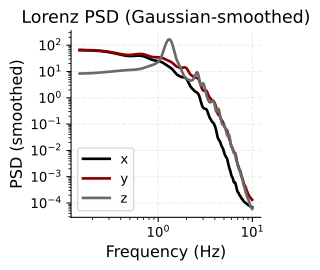
Simulate the Lorenz attractor (\(\sigma=10, \rho=28, \beta=8/3\)) and inspect its power spectral density. The broadband PSD with no sharp spectral peaks confirms chaotic, aperiodic dynamics — a useful test case for autoregressive modeling.

Generate a System with Known Dynamics

The Lorenz coordinates evolve together according to

\[\dot{x}=\sigma(y-x),\qquad \dot{y}=x(\rho-z)-y,\qquad \dot{z}=xy-\beta z.\]

The nonlinear products couple the coordinates. With the parameters below, trajectories repeatedly circulate around two lobes and switch between them without following a fixed repeating cycle. This makes the example different from a sum of stable sinusoids: local motion can be predictable even when long-term phase alignment is not.

nfm.simulation.lorenz integrates these equations with fourth-order Runge-Kutta steps. The call generates 40,000 samples with \(\Delta t=0.005\), using \((\sigma,\rho,\beta)=(10,28,8/3)\) and initial state \((1,1,1)\). The output has shape (samples, 3); transposing it separates the three coordinate arrays.

The sampling rate is \(1/\Delta t=200\) samples per simulation time unit. The plots label frequency in Hz under the convention that one such unit is one second; this is a chosen simulation clock, not a measured physiological timescale. The first 2,000 samples are omitted from the spectral calculation to reduce the effect of the initial approach to the attractor. This trimming applies to data_psd; the later AR fits use the full xs array, including that initial segment.

Show code

Hide code

xs, ys, zs = nfm.simulation.lorenz(n_samples=40000, dt=0.005, sigma=10.0, rho=28.0, beta=8/3, initial_state=(1.0, 1.0, 1.0)).T

fs = 1.0 / 0.005
burn = 2000  # drop transient
data_psd = np.vstack([xs[burn:], ys[burn:], zs[burn:]])  #(3, n_times)

Estimate the Distribution of Power over Frequency

A power spectral density (PSD) describes how the signal’s variance is distributed over frequency. It complements the trajectory view: narrow peaks suggest persistent periodic components, while broader structure indicates activity spread over a range of timescales. For these synthetic coordinates, PSD amplitudes have squared coordinate units per unit frequency; they are not neural recording voltages.

Welch’s method divides each coordinate into overlapping segments, estimates a spectrum for each segment, and averages the estimates. Here the transform length is 4,096 samples, the overlap is 2,048 samples, and the displayed frequency range is 0.1-10 Hz. At the stated sampling rate, the frequency-bin spacing is about 0.049 Hz. Averaging reduces variability between segments, while the finite segment length limits how finely nearby frequencies can be distinguished.

The additional Gaussian smoothing has standard deviation two frequency bins and is applied to each PSD only. It makes broad spectral trends easier to compare; it does not smooth xs, change the AR training signal, or alter the later delay coordinates.

Show code

Hide code

# compute PSD for all three channels 
psds, freqs = mne.time_frequency.psd_array_welch(
    data_psd,
    sfreq=fs,
    fmin=0.1, fmax=10,
    n_fft=4096,
    n_overlap=2048,
    average='mean'
)

# smooth each PSD along frequency axis
Pxx_smooth = gaussian_filter1d(psds[0], sigma=2)
Pyy_smooth = gaussian_filter1d(psds[1], sigma=2)
Pzz_smooth = gaussian_filter1d(psds[2], sigma=2)

Effective window size : 20.480 (s)

Read the Spectra as a Timescale Summary

Both axes are logarithmic. Moving right corresponds to faster variation, and moving upward corresponds to more power per unit frequency. The three curves come from different coordinates of the same coupled system, so different amplitudes or spectral shapes do not imply three independent generators.

Broad spectral content is consistent with the nonperiodic Lorenz trajectory, but a PSD alone does not establish chaos: stochastic processes can also have broad spectra, and smoothing can obscure narrow structure. Here the interpretation comes from the known generating equations as well as the displayed spectrum. This figure summarizes temporal scales; it does not establish the geometry of the reconstructed attractor.

Show code

Hide code

plt.figure(figsize=(3,3))
plt.loglog(freqs, Pxx_smooth, 'k', lw=2, label="x")
plt.loglog(freqs, Pyy_smooth, 'darkred', lw=2, label="y")
plt.loglog(freqs, Pzz_smooth, 'dimgray', lw=2, label="z")
plt.xlabel("Frequency (Hz)")
plt.ylabel("PSD (smoothed)")
plt.title("Lorenz PSD (Gaussian-smoothed)")
plt.grid(True, ls="--", alpha=0.25)
plt.legend()
plt.tight_layout()
plt.show()

AR(p) Order Selection

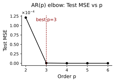
Fit univariate AR models on the \(x\)-component for orders \(p \in \{2,\dots,6\}\). We select \(p\) via test-set MSE and BIC, using an 80/20 train/test split with OLS estimation.

Fit a Linear Baseline from a Single Observed Coordinate

A univariate autoregressive model predicts \(x(t)\) from its own recent history, without observing \(y(t)\) or \(z(t)\):

\[\widehat{x}(t)=b+\sum_{i=1}^{p}a_i x(t-i).\]

nfm.embedding.lag_matrix returns those lagged predictors and their next-sample targets. Each candidate order 2 through 6 is fitted by ordinary least squares on the first 80% of available target rows. Predictions on the later 20% use the observed history at every step. The split is chronological; the test targets are not included in coefficient estimation.

The code records three complementary summaries. Test MSE measures squared one-step error on the later interval. AIC and BIC use training residual variance together with a penalty for the number of fitted parameters; lower values favor a trade-off between fit and complexity. These criteria are linear-model comparisons, not direct measurements of attractor dimension or the number of Lorenz variables.

Although the minimizing orders are calculated, both selection variables are then explicitly set to 3. The remaining linear-model example therefore uses AR(3). The displayed reference is a chosen order, not a guarantee that all three criteria select it automatically.

Show code

Hide code

p_list = list(range(2, 7))
mse_te_list, aic_list, bic_list = [], [], []
params_by_p = {}
splits = {}

for p in p_list:
    X, y = nfm.embedding.lag_matrix(xs, order=p)
    N = len(y)
    ntr = int(0.8 * N)
    X_tr, y_tr = X[:ntr], y[:ntr]
    X_te, y_te = X[ntr:], y[ntr:]
    _ar_fit = nfm.models.AR(order=p).fit(xs[:p + ntr])
    w = np.r_[_ar_fit.intercept, _ar_fit.coefficients]
    yhat_tr = (np.column_stack([np.ones(len(X_tr)), X_tr]) @ w)
    yhat_te = (np.column_stack([np.ones(len(X_te)), X_te]) @ w)
    _metrics = nfm.models.prediction_metrics(y_te, yhat_te)
    (mse_te, _, _) = _metrics.mse, _metrics.mae, _metrics.correlation
    _criteria = _ar_fit.information_criteria(xs[:p + ntr])
    (aic, bic) = _criteria["aic"], _criteria["bic"]
    mse_te_list.append(mse_te); aic_list.append(aic); bic_list.append(bic)
    params_by_p[p] = w
    splits[p] = (ntr, y, yhat_tr, yhat_te)

best_p_by_mse = p_list[int(np.argmin(mse_te_list))]
best_p_by_bic = p_list[int(np.argmin(bic_list))]

best_p_by_mse = 3
best_p_by_bic = 3

Interpret the Order-Error Curve

A falling curve means that extra lagged observations improve local prediction; a flattening curve indicates diminishing improvement over this tested range. Densely sampled smooth dynamics can yield very small one-step errors because adjacent observations are close in time. That success need not translate into a faithful free-running attractor.

The vertical line marks the chosen order 3. Compare its error with neighboring orders rather than reading the line’s label as an additional optimization result. If the test curve is used to choose settings for a predictive study, an additional untouched interval is needed for a final performance estimate. Here the curve introduces the linear baseline used in the subsequent diagnostics.

Show code

Hide code

fig, ax = plt.subplots(figsize=(4,3))
ax.plot(p_list, mse_te_list, marker='o', color=color_main, lw=1.5, ms=5)
ax.axvline(best_p_by_mse, linestyle='--', color=color_alt, linewidth=1)
ax.text(best_p_by_mse, ax.get_ylim()[1]*0.95, f"best p={best_p_by_mse}",
        ha='center', va='top', color=color_alt, fontsize=11)

sf = ScalarFormatter(useMathText=True)
sf.set_powerlimits((-3, 3))   # switch to sci notation outside this range
ax.yaxis.set_major_formatter(sf)
ax.ticklabel_format(axis='y', style='sci', scilimits=(-3, 3))
ax.yaxis.get_offset_text().set_size(10)  # the “×10^−4” offset text
nfm.plotting.prettify(ax, title="AR(p) elbow: Test MSE vs p", xlabel="Order p", ylabel="Test MSE")
plt.tight_layout(); plt.show()

Fitted Coefficients & One-Step Prediction

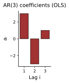
The AR(\(p\)) coefficient magnitudes show how much each lag contributes. We then evaluate the model’s one-step-ahead forecast against held-out data.

Understand the Lag Weights

Each bar is the fitted coefficient for one preceding sample. The intercept is stored in w[0] and is not shown. Positive and negative weights combine to reproduce local increases, decreases, and curvature in the waveform. Because neighboring samples are strongly dependent, large weights may partly cancel; the height of one bar is not the strength of a separate dynamical source.

These coefficients describe a single linear approximation across the training interval. The actual Lorenz equations are nonlinear, so a useful next-sample approximation does not imply that this fixed linear rule captures every region of the attractor equally well.

Show code

Hide code

p_use = best_p_by_bic
w = params_by_p[p_use]
fig, ax = plt.subplots(figsize=(2,3))
bars = ax.bar(np.arange(1, p_use+1), w[1:], color=color_alt, edgecolor=color_main, alpha=0.8)
nfm.plotting.prettify(ax, title=f"AR({p_use}) coefficients (OLS)", xlabel="Lag i", ylabel="aᵢ")
plt.tight_layout(); plt.show()

Distinguish One-Step Prediction from Free-Running Simulation

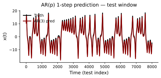
Every prediction in this overlay is computed from the actual preceding observations in the test segment. The output is not fed back to generate the next test prediction. This answers whether the fitted linear rule approximates local motion when the current observed history is supplied, not whether it can sustain the attractor alone.

The plotting cell adds 1 to the observed trace to separate it visually from the prediction. This is a display offset, not a measured model bias; residuals and scatter comparisons use the unshifted values. The horizontal axis is test-sample index, with one sample corresponding to 0.005 simulation time units. The final win assignment displays the full available test interval rather than just its first 1,500 samples.

Look for agreement in peak timing and waveform shape. The following diagnostics then examine errors that can be difficult to see in overlapping traces.

Show code

Hide code

ntr, y_all, yhat_tr, yhat_te = splits[p_use]
X, y = nfm.embedding.lag_matrix(xs, order=p_use)
fig, ax = plt.subplots(figsize=(6,3))
win = slice(ntr, min(ntr+1500, len(y)))
win = slice(ntr, len(y))   # all available test samples

ax.plot(y[win]+1, color=color_main, lw=2, label="Truth")
ax.plot(yhat_te[:win.stop-win.start], color=color_alt, lw=2, label=f"AR({p_use}) pred")
nfm.plotting.prettify(ax, title="AR(p) 1-step prediction — test window", xlabel="Time (test index)", ylabel="x(t)", add_legend=True)
plt.tight_layout(); plt.show()

Residual Diagnostics

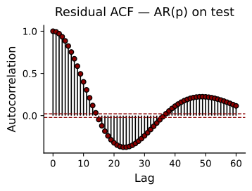
If the AR model captures all linear dependence, residuals should be white noise. The ACF of test residuals should fall within the 95% confidence bands (\(\pm 1.96/\sqrt{N}\)). Significant autocorrelation at low lags signals model misspecification.

Read Structure in the Prediction Errors

The residual \(e(t)=x(t)-\widehat{x}(t)\) records what the linear model leaves unexplained. Its autocorrelation asks whether an error tends to be followed by related errors. Lag zero is 1 by definition; sustained structure at positive lags indicates that the errors retain temporal organization, even if their absolute amplitude is small.

The plot extends to 60 samples, or 0.3 simulation time units. A slowly decaying or oscillating pattern suggests that a fixed linear predictor has not removed all dependence at those timescales. This motivates inspecting a model that can change its local rule rather than relying on one-step MSE alone.

The dashed \(\pm1.96/\sqrt{N}\) lines are an approximate pointwise white-noise reference, not a simultaneous 95% band for all 60 lags. Uncorrelated errors are also not necessarily independent or Gaussian. Read the ACF as a diagnostic of remaining dependence, not a proof that the nonlinear generating dynamics have been recovered.

Show code

Hide code

resid_te = y[ntr:] - yhat_te
acf_vals = acf(resid_te, nlags=60)
N_te = len(resid_te)
bound = 1.96 / np.sqrt(max(N_te,1))

fig, ax = plt.subplots(figsize=(4,3))
markerline, stemlines, baseline = ax.stem(range(len(acf_vals)), acf_vals, basefmt=" ")

# Customize stem plot colors
plt.setp(stemlines, color=color_main, linewidth=1.2)
plt.setp(markerline, marker='o', markersize=5,
         markeredgecolor=color_main, markerfacecolor=color_alt)

# Add confidence bounds
ax.axhline(bound, linestyle='--', color=color_alt, linewidth=1)
ax.axhline(-bound, linestyle='--', color=color_alt, linewidth=1)

nfm.plotting.prettify(ax, title="Residual ACF — AR(p) on test", xlabel="Lag", ylabel="Autocorrelation")
plt.tight_layout()
plt.show()

Check Pointwise Agreement without a Display Offset

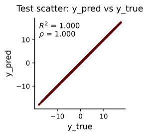
Each point pairs an observed test value with its prediction at the same time. Perfect predictions lie on the diagonal identity line. A displaced cloud reveals bias, a different slope reveals a scale mismatch, and spread around the line reveals samplewise error.

Pearson correlation \(\rho\) describes linear covariation and can be high even with a gain or offset error. The coefficient of determination,

\[R^2=1-\frac{\sum_t(x(t)-\widehat{x}(t))^2} {\sum_t(x(t)-\overline{x})^2},\]

additionally compares squared error with the test-mean baseline. It is 1 for exact predictions and can be negative for sufficiently poor predictions. Both annotations describe the same one-step protocol as the overlay. Neither measures whether a separately simulated trajectory occupies the correct attractor.

Show code

Hide code

y_true = y[ntr:]
y_pred = yhat_te
fig, ax = plt.subplots(figsize=(3,3))
ax.scatter(y_true, y_pred, c=color_alt, alpha=0.35, s=10, edgecolors="none")
# identity line
vmin = min(np.min(y_true), np.min(y_pred))
vmax = max(np.max(y_true), np.max(y_pred))
ax.plot([vmin, vmax], [vmin, vmax], color=color_main, lw=1)

# R² and corr
yt = y_true - np.mean(y_true)
yp = y_pred - np.mean(y_pred)
corr = float((yt @ yp) / np.sqrt((yt @ yt) * (yp @ yp) + 1e-12))
ss_res = np.sum((y_true - y_pred)**2)
ss_tot = np.sum((y_true - np.mean(y_true))**2)
r2 = 1 - ss_res / (ss_tot + 1e-12)
ax.text(0.05, 0.95, f"$R^2$ = {r2:.3f}\n$\\rho$ = {corr:.3f}",
        transform=ax.transAxes, ha='left', va='top', fontsize=11,
        bbox=dict(facecolor="white", edgecolor="none", alpha=0.7, boxstyle="round"))

ax.set_aspect('equal', adjustable='box')
nfm.plotting.prettify(ax, title="Test scatter: y_pred vs y_true", xlabel="y_true", ylabel="y_pred")
plt.tight_layout(); plt.show()

Threshold AR & Attractor Reconstruction

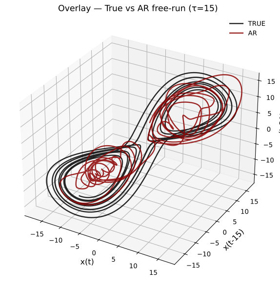
A linear AR model captures one-step dynamics but cannot reproduce the Lorenz attractor’s geometry under free-run simulation. We fit a Threshold AR (TAR) model, which switches regimes based on a delay variable, then free-run simulate and apply time-delay embedding (\(m=3, \tau=15\)) to compare the reconstructed attractors.

Allow the Dynamical Rule to Depend on the Recent State

A threshold autoregressive model (TAR) fits two linear predictors and chooses between them according to a delayed signal value. Here each predictor has order 8, and the switch is determined by whether \(x(t-1)\leq0\) or \(x(t-1)>0\). This adds a simple form of nonlinearity: the same set of lagged observations is interpreted by different coefficient vectors in different parts of the scalar state. The threshold does not provide an observed label for the full three-dimensional Lorenz state.

This cell generates a new 12,000-sample trajectory using the Lorenz function’s defaults, including \(\Delta t=0.005\) and the same system parameters. It does not reuse the preceding 40,000-sample array. The first 80% of lag-matrix targets fits the two regimes by least squares; the remaining interval supplies the comparison trace. No initial transient is explicitly removed from this fit.

Simulation begins with the eight observed samples immediately before that comparison interval, ordered newest first. Subsequent steps use generated history rather than repeated observed-history refreshes. At each step, the simulator adds a residual sampled from the fitted regime’s training residuals. Thus the result is a residual-bootstrap simulation, not a deterministic integration of the Lorenz equations. seed=42 makes that sampling reproducible.

match_reference=true_test then matches the generated trace’s mean and standard deviation to the observed comparison trace. This uses information from that interval for distribution-matched geometric visualization; it must not be interpreted as a fully held-out, amplitude-calibrated forecast evaluation.

Show code

Hide code

xs, ys, zs = nfm.simulation.lorenz(n_samples=12000).T
p_use, d_use = 8, 1
ntr = int(0.8 * (len(xs) - p_use))
tar = nfm.models.TAR(order=p_use, delay_samples=d_use, threshold=0.0).fit(xs[:p_use + ntr])
true_test = xs[p_use + ntr:]
t_x_start_test = p_use + ntr
init = [xs[t_x_start_test - i] for i in range(1, p_use + 1)]
n_steps = len(true_test)
x_tar = tar.simulate(init, n_samples=n_steps, seed=42, match_reference=true_test)
tau = 15
X3_true = nfm.embedding.delay(np.asarray(true_test, dtype=np.float32), dimension=3, tau_samples=tau)
X3_tar = nfm.embedding.delay(np.asarray(x_tar, dtype=np.float32), dimension=3, tau_samples=tau)

Compare the Geometry of Observed and Generated Trajectories

Both scalar traces are mapped to the same delayed coordinates:

\[\mathbf{z}(t)=[x(t),\;x(t-\tau),\;x(t-2\tau)].\]

The embedding dimension is 3 and the delay is 15 samples, corresponding to 0.075 simulation time units. Each point therefore spans 30 samples of history, and a trace of length \(N\) contributes \(N-30\) points. This coordinate delay is distinct from the TAR’s one-sample switching delay: one defines the visualization, while the other determines which predictor generates a sample.

The black trajectory embeds the observed Lorenz \(x\) coordinate, not the original \((x,y,z)\) state. The dark-red trajectory embeds the amplitude-matched TAR simulation. Although the legend abbreviates it as AR, the simulated model is the two-regime TAR fitted above.

Compare overall extent, folds, circulation, and occupancy rather than expecting point-by-point phase alignment. A chaotic reference and a residual-driven simulation can visit similar regions at different times. Matching the first two amplitude moments does not force their detailed geometry to agree, but visual overlap alone is also not a quantitative demonstration of equivalent dynamics or topology. This cell plots trajectories; it does not fit a torus surface or calculate persistent homology.

Show code

Hide code

# Overlay
n_overlay = min(len(X3_true), len(X3_tar))
X3_true_m = X3_true[:n_overlay]
X3_tar_m  = X3_tar[:n_overlay]

plt.rcParams.update({
    "figure.dpi": 120, "font.size": 12,
    "axes.spines.top": False, "axes.spines.right": False,
    "axes.grid": True, "grid.alpha": 0.25
})

fig = plt.figure(figsize=(8,6), constrained_layout=True)
ax = fig.add_subplot(111, projection='3d')

ax.plot(X3_true_m[:,0], X3_true_m[:,1], X3_true_m[:,2], color = 'black',label="TRUE", alpha=0.85)
ax.plot(X3_tar_m[:,0],  X3_tar_m[:,1],  X3_tar_m[:,2],  color = 'darkred',label="AR", alpha=0.85)
ax.set_title(f"Overlay — True vs AR free-run (τ={tau})")
ax.set_xlabel("x(t)"); ax.set_ylabel(f"x(t-{tau})"); ax.set_zlabel(f"x(t-{2*tau})")

ax.legend(frameon=False)
plt.show()

What the Example Demonstrates

The tutorial separates three questions that are easy to conflate:

• What timescales are present? The coordinate PSDs summarize spectral content, but do not by themselves identify chaos or reconstruct the attractor.

• Can the next sample be predicted? The linear AR error curve, waveform, residual ACF, and scatter characterize short-horizon prediction when the observed lag history is available.

• What happens when the model drives itself? The TAR simulation tests a state-dependent rule without ongoing history refreshes, and its delay embedding gives a complementary geometric view.

A strong one-step score is not a substitute for inspecting generated dynamics. Conversely, an appealing attractor overlay does not establish correct pointwise forecasting. Keep the fitting interval, simulation protocol, amplitude matching, and embedding settings explicit when comparing these results or adapting the workflow.

For oscillatory signals with controlled mode structure, continue with Intrinsic vs. Embedding Dimensionality. For examples with filtering, envelope normalization, and multiple recording channels, see Monkey V1 LFP, Mice Hippocampus EEG, and Mice Hippocampus LFP.