Mice Hippocampus LFP

A neural recording is observed as a single waveform, but its temporal relationships can be represented as a trajectory in a reconstructed state space. This tutorial uses a mice hippocampus LFP recording to connect two views of the same signal: an autoregressive model of its local dynamics and the geometry of its delay coordinates.

The workflow moves from loading and processing a channel to fitting a classical AR model, inspecting its prediction errors, and comparing observed and reconstructed trajectories. Time-window, delay, and channel comparisons then show which features of the geometry depend on the chosen view. Black curves represent the processed recording; dark-red curves represent the model reconstruction.

The aim is to understand what the model reproduces and how to interpret the resulting geometry, not simply to maximize a prediction score. A loop or torus-like appearance is a useful geometric observation, but a three-dimensional picture alone does not determine topology or count independent generators. These examples use a fitted linear AR model; they do not require training DeepLagField.

1. Set Up the Notebook

Install the package with its tutorials dependencies as described in Installation, then run the cells in order. neuralfieldmanifold is imported as nfm. NumPy handles arrays, Matplotlib displays the comparisons, and the shared plotting style keeps figures consistent across the tutorial.

The complete analysis includes multiple recording channels, so it requires the recording file(s) described below. The small bundled samples used in Getting Started are suitable for learning the API but do not contain every channel needed here. The website displays saved results; opening a page does not run the analysis or require access to the recording.

Show code

Hide code

import neuralfieldmanifold as nfm

Show code

Hide code

import neuralfieldmanifold as nfm
import matplotlib.pyplot as plt
from pathlib import Path
import os
color_main, color_alt = "black", "darkred"
import numpy as np
import mne
import os
from scipy import signal
from scipy.signal import hilbert, butter, filtfilt, spectrogram
from scipy.ndimage import gaussian_filter, gaussian_filter1d
from matplotlib.ticker import ScalarFormatter
from statsmodels.tsa.stattools import acf
import matplotlib.pyplot as plt





import warnings
warnings.simplefilter(action='ignore', category=FutureWarning)

nfm.plotting.set_style()

from matplotlib_inline.backend_inline import set_matplotlib_formats
set_matplotlib_formats("svg", "retina")

2. Assemble the Reconstruction Pipeline

The helper functions separate three tasks: preparing a signal, estimating its dynamics, and comparing observed and reconstructed trajectories. Signal processing is handled by nfm.preprocessing; the autoregressive design matrix comes from nfm.embedding.lag_matrix; and nfm.models.AR estimates the coefficients by ordinary least squares.

An autoregressive model of order \(p\) predicts the next sample from the previous \(p\) samples:

\[\widehat{x}(t)=b+\sum_{i=1}^{p}a_i x(t-i).\]

The intercept \(b\) accounts for a constant offset. The coefficients \(a_i\) describe how recent observations combine to predict the next value. Fitting minimizes squared prediction error on the training segment. The returned w stores the intercept first, followed by coefficients from lag 1 to lag \(p\).

Three settings have different roles throughout this tutorial: AR order \(p\) controls the predictor’s memory, embedding dimension \(m\) controls the number of plotted coordinates, and delay \(\tau\) controls the spacing between those coordinates. Neither \(p\) nor \(m\) is, by itself, a measurement of the number of independent oscillatory modes.

Show code

Hide code

def bandpass_filter(x, Fs, low, high, order=4):
    return nfm.preprocessing.bandpass(x, sampling_rate_hz=Fs, band_hz=(low, high), order=order)

def envelope_normalize(x, fs, fband=(15, 30), env_lp_hz=5.0, eps=1e-6):
    return nfm.preprocessing.envelope_normalize(x, sampling_rate_hz=fs, band_hz=fband, lowpass_hz=env_lp_hz, epsilon=eps)

def process_signal(LFP, chan, Fs, time_window, 
                   notch_freq=50, notch_Q=30,
                   bandpass_low=80, bandpass_high=140,
                   fband=(1, 80), env_lp_hz=3.0,
                   target_Fs=500):
    """Process LFP signal with notch filter, bandpass, envelope normalization, and downsampling."""
    config = nfm.preprocessing.PreprocessConfig(
        notch_hz=notch_freq, notch_quality=notch_Q,
        band_hz=(bandpass_low, bandpass_high),
        envelope_band_hz=fband, envelope_lowpass_hz=env_lp_hz,
        output_rate_hz=Fs / int(np.floor(Fs / target_Fs)) if Fs > target_Fs else None,
    )
    processed = nfm.preprocessing.process(LFP[time_window, chan], sampling_rate_hz=Fs, config=config)
    return processed.signal, processed.bandpassed, processed.sampling_rate_hz


def fit_ar_model(xs, Fs, p=4, train_frac=0.9, refresh_every=10):
    X, y = nfm.embedding.lag_matrix(xs, order=p)
    ntr = int(train_frac * len(y))
    X_tr, y_tr = X[:ntr], y[:ntr]
    _ar_fit = nfm.models.AR(order=p).fit(xs[:p + ntr])
    w = np.r_[_ar_fit.intercept, _ar_fit.coefficients]
    N_te = len(y) - ntr
    t0 = p + ntr
    true_test = xs[t0 : t0 + N_te]
    yhat_ctrl = nfm.models.ARFit(w[0], w[1:]).forecast(xs, start_sample=t0, n_samples=N_te, refresh_samples=refresh_every)
    full_pred = nfm.models.ARFit(w[0], w[1:]).forecast(xs, start_sample=p, n_samples=len(xs)-p, refresh_samples=refresh_every)
    xs_pred_full = np.concatenate([xs[:p], full_pred])
    _metrics = nfm.models.prediction_metrics(true_test, yhat_ctrl)
    (mse, mae, corr) = _metrics.mse, _metrics.mae, _metrics.correlation
    return {
        'w': w, 'p': p, 'ntr': ntr, 'y': y, 'true_test': true_test,
        'yhat_ctrl': yhat_ctrl, 'xs_pred_full': xs_pred_full, 't0': t0,
        'mse': mse, 'mae': mae, 'corr': corr, 'refresh_every': refresh_every
    }

3. Load a Channel from the Recording

Set NFM_MOUSE_DATA_FILE to the NumPy recording used below. The loader expects (channels, samples), selects zero-based channel_id = 1, and obtains a one-dimensional waveform. The acquisition rate is set explicitly to 20,000 Hz; the array’s shape does not itself specify a sampling rate.

The single-channel example uses the first five seconds, or 100,000 acquired samples. It reshapes the selected waveform to (samples, 1) for the processing helper. The later channel comparison reloads the full channel-by-sample array and transposes it for that same helper. Keeping these axis conventions explicit prevents selecting a time point where a channel was intended.

The recording path can be changed without changing the workflow, but its sampling rate, available channels, and duration must match the parameters supplied to the analysis. All sample-index-to-time conversions after processing use the returned rate Fs, not the original acquisition rate.

Show code

Hide code

filename = Path(os.environ.get("NFM_MOUSE_DATA_FILE", "data/eke003_spont_250818_175844.npy"))
channel_id = 1
raw_lfp = np.load(filename)[channel_id]
fs_original = 20000

print(f"Loaded LFP: {raw_lfp.shape} samples at {fs_original} Hz")

Loaded LFP: (10841760,) samples at 20000 Hz

4. Prepare the Signal for Dynamical Reconstruction

Processing defines which activity the subsequent model describes. The following call, rather than the helper’s default arguments, sets the analysis band to 1-20 Hz. The steps run in this order:

1. Notch at 50 Hz, with quality factor 30, to attenuate a narrow line-frequency component. This example’s setting is not a universal choice for recordings acquired under different line frequencies.

2. Bandpass at 1-20 Hz with a fourth-order Butterworth design. This emphasizes the temporal activity being reconstructed while reducing slow drift and activity outside that band.

3. Decimate from 20 kHz to 500 Hz. The integer factor is 40. Decimation includes an anti-alias filter; it is not simply taking every fortieth sample. The retained band is well below the new 250 Hz Nyquist frequency. This rate is used for the low-frequency reconstruction, not for retaining the full acquisition bandwidth.

4. Normalize by a smoothed amplitude envelope. The normalization stage filters at 1-80 Hz, computes the Hilbert amplitude, smooths the envelope with a 3 Hz lowpass, and divides by that envelope plus a small positive constant. Multiplication by the median envelope retains an overall signal scale.

Envelope normalization reduces slow changes in trajectory size so that phase relationships are easier to compare. It is not a z-score, and its output is not an unmodified voltage trace. The 1-80 Hz envelope band does not restore content removed by the earlier bandpass; division by the time-varying envelope can itself modify the spectrum.

xs is the final normalized signal used for modeling. Despite its name, xs_raw is the filtered, pre-envelope signal returned by the helper, not the untouched recording. Filtering is zero-phase and uses samples on both sides of a point, making this an offline analysis. Short intervals near filter boundaries should be interpreted with care.

Show code

Hide code

snippet_sec = 5
time_window = np.arange(int(snippet_sec * fs_original))

# Reshape raw_lfp to (samples, channels) format for process_signal
LFP = raw_lfp.reshape(-1, 1)

xs, xs_raw, Fs = process_signal(LFP, chan=0, Fs=fs_original, time_window=time_window,
                                 bandpass_low=1, bandpass_high=20,
                                 fband=(1, 80), env_lp_hz=3.0,
                                 target_Fs=500)

time = np.arange(len(xs)) / Fs
print(f"Processed signal: {len(xs)} samples at {Fs} Hz")

Processed signal: 2500 samples at 500.0 Hz

5. Explore How Much Lag History Is Needed

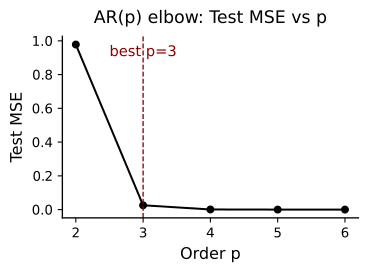
The order sweep fits AR models with \(p=2,\ldots,6\). For each order, nfm.embedding.lag_matrix pairs a row of past observations with its next-sample target. The first 10% of target rows is used for fitting, and the remaining rows are used for the displayed error curve. This is a chronological split, not a random shuffle of samples.

The curve reports one-step test MSE: every test prediction receives the actual preceding observations. A flattening curve indicates that adding lags yields little further improvement for this recording and interval. Increasing order gives the model more flexibility but does not automatically reveal more independent oscillations.

The minimum-MSE order is computed first, after which best_p_by_mse is explicitly set to 3. Both the reference line and the subsequent single-channel reconstruction use AR(3). Read the line as the example’s chosen order rather than an automatically accepted optimum.

This is an exploratory order comparison. If the curve is used to tune a model for a new prediction study, choose the order within the training data and reserve a separate interval for the final performance estimate.

Show code

Hide code

# Sweep AR orders for elbow plot
p_list = list(range(2, 7))
mse_te_list = []
for p in p_list:
    X, y_temp = nfm.embedding.lag_matrix(xs, order=p)
    ntr_temp = int(0.1 * len(y_temp))
    X_tr, y_tr = X[:ntr_temp], y_temp[:ntr_temp]
    X_te, y_te = X[ntr_temp:], y_temp[ntr_temp:]
    _ar_fit = nfm.models.AR(order=p).fit(xs[:p + ntr_temp])
    w_temp = np.r_[_ar_fit.intercept, _ar_fit.coefficients]
    yhat_te = (np.column_stack([np.ones(len(X_te)), X_te]) @ w_temp)
    _metrics = nfm.models.prediction_metrics(y_te, yhat_te)
    (mse_te, _, _) = _metrics.mse, _metrics.mae, _metrics.correlation
    mse_te_list.append(mse_te)

best_p_by_mse = p_list[int(np.argmin(mse_te_list))]

def plot_mse_elbow(p_list, mse_list, best_p, color_main="black", color_alt="darkred"):
    fig, ax = plt.subplots(figsize=(4, 3))
    ax.plot(p_list, mse_list, marker='o', color=color_main, lw=1.5, ms=5)
    ax.axvline(best_p, linestyle='--', color=color_alt, linewidth=1)
    ax.text(best_p, ax.get_ylim()[1]*0.95, f"best p={best_p}", ha='center', va='top', color=color_alt, fontsize=11)
    sf = ScalarFormatter(useMathText=True)
    sf.set_powerlimits((-3, 3))
    ax.yaxis.set_major_formatter(sf)
    ax.ticklabel_format(axis='y', style='sci', scilimits=(-3, 3))
    ax.yaxis.get_offset_text().set_size(10)
    nfm.plotting.prettify(ax, title="AR(p) elbow: Test MSE vs p", xlabel="Order p", ylabel="Test MSE")
    plt.tight_layout()
    plt.show()

best_p_by_mse = 3

plot_mse_elbow(p_list, mse_te_list, best_p_by_mse)

6. Fit the Model and Reconstruct the Held-Out Interval

The main example fits AR(3) on the initial 10% of available target rows and evaluates on the later 90%. The coefficients remain fixed after fitting; they are not re-estimated as the test trace advances.

Unlike the order sweep, this step uses a recursive forecast with observed-history refreshes every 10 samples (20 ms at 500 Hz). At each refresh the predictor receives the actual preceding lag values. Within that block, it feeds its predictions back into the model. This tests short stretches of model evolution while limiting accumulated drift. It is neither an uninterrupted free run nor a one-step prediction at every sample.

true_test and yhat_ctrl are aligned observed and predicted test arrays. The printed MSE measures squared amplitude error, while the correlation measures waveform covariation. Their protocol differs from the one-step order curve, so they need not have the same error. xs_pred_full additionally reconstructs the complete processed interval for visualization; its initial model history is copied from the recording.

Show code

Hide code

ar_results = fit_ar_model(xs, Fs, p=3, train_frac=0.1, refresh_every=10)

w = ar_results['w']
p_use = ar_results['p']
ntr = ar_results['ntr']
y = ar_results['y']
true_test = ar_results['true_test']
yhat_ctrl = ar_results['yhat_ctrl']
xs_pred_full = ar_results['xs_pred_full']
REFRESH_EVERY = ar_results['refresh_every']

print(f"AR({p_use}): MSE={ar_results['mse']:.6f}, corr={ar_results['corr']:.3f}")

AR(3): MSE=192.180213, corr=0.990

Interpret the Fitted Coefficients

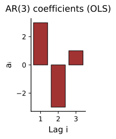
Each bar is the coefficient multiplying one lagged sample. Positive coefficients reinforce that sample’s contribution; negative coefficients subtract it. Together, these weights can describe oscillation, decay, or a mixture of temporal patterns. The intercept is not included in this bar plot.

Read the coefficients as a group rather than treating a large bar as a separate oscillation. Neighboring samples of a filtered signal can be highly correlated, so large positive and negative coefficients may partly cancel. Oscillatory modes are associated with complex-conjugate poles of the fitted AR model, not individual coefficients. The pole analysis in the dimensionality tutorial develops that connection.

Show code

Hide code

def plot_ar_coefficients(w, p, color_main="black", color_alt="darkred"):
    fig, ax = plt.subplots(figsize=(2, 3))
    ax.bar(np.arange(1, p+1), w[1:], color=color_alt, edgecolor=color_main, alpha=0.8)
    nfm.plotting.prettify(ax, title=f"AR({p}) coefficients (OLS)", xlabel="Lag i", ylabel="aᵢ")
    plt.tight_layout()
    plt.show()

plot_ar_coefficients(w, p_use)

7. Compare the Reconstructed and Observed Waveforms

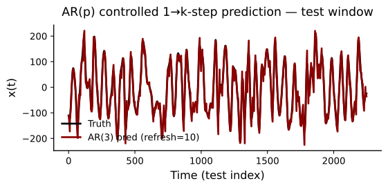
The overlay shows whether the fitted model follows the timing and shape of the processed recording. Between history refreshes, each prediction becomes an input to the next prediction. Errors can therefore accumulate within a block even though the model is periodically re-anchored to observed data.

The prediction function below adds 1 to the observed trace for display and leaves the prediction unshifted. That vertical separation is a plotting offset, not an estimated bias. Compare peaks, troughs, and temporal alignment here; use the residual and scatter plots for amplitude error. The horizontal axis is the test-sample index, so dividing by Fs gives elapsed seconds within the test interval.

Accurate short-horizon reconstruction is useful evidence that the AR model captures local dependence. It does not yet establish that an autonomous simulation would reproduce the signal’s longer-term geometry.

Show code

Hide code

def plot_prediction(y_true, y_pred, p, refresh, color_main="black", color_alt="darkred"):
    fig, ax = plt.subplots(figsize=(6, 3))
    ax.plot(y_true + 1, color=color_main, lw=2, label="Truth")
    ax.plot(y_pred, color=color_alt, lw=2, label=f"AR({p}) pred (refresh={refresh})")
    nfm.plotting.prettify(ax, title="AR(p) controlled 1→k-step prediction — test window", xlabel="Time (test index)", ylabel="x(t)", add_legend=True)
    plt.tight_layout()
    plt.show()

plot_prediction(y[ntr:], yhat_ctrl, p_use, REFRESH_EVERY)

Examine What the Model Leaves Unexplained

A residual is the observed value minus its prediction:

\[e(t)=x(t)-\widehat{x}(t).\]

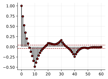
The residual autocorrelation function (ACF) asks whether errors separated by a given number of samples still vary together. Lag zero is always 1. Repeated structure at nonzero lags means that the reconstructed waveform leaves temporal dependence unexplained; an oscillating ACF can reveal a residual rhythmic component that is not obvious in a small waveform overlay. Convert an ACF lag to seconds by dividing it by Fs.

The dashed lines are the familiar white-noise reference \(\pm1.96/\sqrt{N}\), where \(N\) is the number of residuals. They are an approximate pointwise guide, not simultaneous confidence bounds across all lags. These residuals also come from periodically refreshed recursive predictions rather than solely one-step innovations. Interpret the overall ACF pattern alongside the prediction protocol, rather than requiring every stem to lie inside the dashed lines.

Show code

Hide code

def plot_residual_acf(resid, nlags=60, color_main="black", color_alt="darkred"):
    acf_vals = acf(resid, nlags=nlags)
    bound = 1.96 / np.sqrt(max(len(resid), 1))
    fig, ax = plt.subplots(figsize=(4, 3))
    markerline, stemlines, baseline = ax.stem(range(len(acf_vals)), acf_vals, basefmt=" ")
    plt.setp(stemlines, color=color_main, linewidth=1.2)
    plt.setp(markerline, marker='o', markersize=5, markeredgecolor=color_main, markerfacecolor=color_alt)
    ax.axhline(bound, linestyle='--', color=color_alt, linewidth=1)
    ax.axhline(-bound, linestyle='--', color=color_alt, linewidth=1)
    plt.tight_layout()
    plt.show()

resid_te = y[ntr:] - yhat_ctrl
plot_residual_acf(resid_te)

Show code

Hide code

REFRESH_EVERY

10

Separate Timing Agreement from Amplitude Agreement

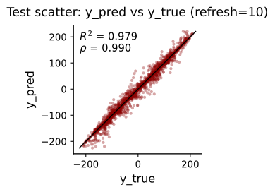
In the scatter plot, each point pairs one observed test value with its prediction at the same time. Perfect predictions lie on the identity line. A change in slope indicates a gain mismatch, a displaced cloud indicates an offset, and broad scatter indicates samplewise error. Unlike the waveform overlay, the observations are not shifted here.

The two annotations describe different aspects of agreement. Pearson correlation \(\rho\) measures linear covariation and can remain high despite a scale or offset mismatch. The coefficient of determination,

\[R^2=1-\frac{\sum_t(x(t)-\widehat{x}(t))^2} {\sum_t(x(t)-\overline{x})^2},\]

compares squared error with predicting the observed test mean. It is 1 for a perfect reconstruction and can be negative when the prediction is worse than that mean baseline. Both quantities are evaluated on the original prediction amplitudes, before the matching used in the geometry plots.

Show code

Hide code

def plot_scatter(y_true, y_pred, refresh, color_main="black", color_alt="darkred"):
    fig, ax = plt.subplots(figsize=(3, 3))
    ax.scatter(y_true, y_pred, c=color_alt, alpha=0.35, s=10, edgecolors="none")
    vmin, vmax = min(np.min(y_true), np.min(y_pred)), max(np.max(y_true), np.max(y_pred))
    ax.plot([vmin, vmax], [vmin, vmax], color=color_main, lw=1)
    yt = y_true - np.mean(y_true)
    yp = y_pred - np.mean(y_pred)
    corr = float((yt @ yp) / np.sqrt((yt @ yt) * (yp @ yp) + 1e-12))
    ss_res = np.sum((y_true - y_pred)**2)
    ss_tot = np.sum((y_true - np.mean(y_true))**2)
    r2 = 1 - ss_res / (ss_tot + 1e-12)
    ax.text(0.05, 0.95, f"$R^2$ = {r2:.3f}\n$\\rho$ = {corr:.3f}",
            transform=ax.transAxes, ha='left', va='top', fontsize=11,
            bbox=dict(facecolor="white", edgecolor="none", alpha=0.7, boxstyle="round"))
    ax.set_aspect('equal', adjustable='box')
    nfm.plotting.prettify(ax, title=f"Test scatter: y_pred vs y_true (refresh={refresh})", xlabel="y_true", ylabel="y_pred")
    plt.tight_layout()
    plt.show()

plot_scatter(y[ntr:], yhat_ctrl, REFRESH_EVERY)

8. Turn Temporal Relationships into a Spatial Trajectory

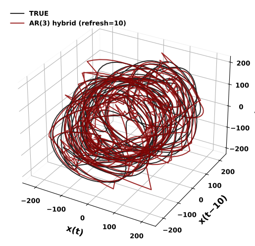
A delay embedding places a sample and two delayed observations in the same three-dimensional point:

\[\mathbf{z}(t)=\left[x(t),\;x(t-\tau),\;x(t-2\tau)\right].\]

Advancing \(t\) traces a curve. For a simple oscillation, delayed coordinates represent different phases and can open a loop. Multiple sustained oscillations can produce richer, torus-like structure when their phases are sufficiently independent and the delays resolve them. Noise, changing amplitudes, finite observation time, and the choice of coordinates affect what is visible; a torus is not guaranteed by choosing a particular AR order.

Here \(m=3\) and \(\tau=10\) samples, or 20 ms at 500 Hz. nfm.embedding.delay returns rows ordered in time with the newest sample first. A segment of \(N\) samples produces \(N-2\tau\) points, because the earliest samples do not have a complete delayed history. The delay is supplied explicitly in this example, not selected by an optimization routine.

Before plotting, the predicted trace is shifted and scaled to match the test trace’s mean and standard deviation. This helps compare shape and temporal organization separately from overall amplitude. It uses the observed comparison interval and is not part of the previously reported prediction accuracy. Black is the processed recording and dark red is the amplitude-matched, periodically refreshed reconstruction. No torus surface is fitted in this cell.

Show code

Hide code

def plot_state_space(X3_true, X3_pred, p, tau, refresh, color_true="black", color_pred="darkred"):
    from matplotlib.ticker import MaxNLocator
    fig = plt.figure(figsize=(8, 6))
    ax = fig.add_subplot(111, projection='3d')
    ax.plot(X3_true[:,0], X3_true[:,1], X3_true[:,2], label="TRUE", color=color_true, alpha=0.85, lw=1.5)
    ax.plot(X3_pred[:,0], X3_pred[:,1], X3_pred[:,2], label=f"AR({p}) hybrid (refresh={refresh})", color=color_pred, alpha=0.85, lw=1.5)

    # Bold axis labels (LaTeX)
    ax.set_xlabel(r"$\mathbf{x(t)}$", labelpad=8, fontsize=13)
    ax.set_ylabel(f"$\\mathbf{{x(t\\!-\\!{tau})}}$", labelpad=8, fontsize=13)
    ax.set_zlabel(f"$\\mathbf{{x(t\\!-\\!{2*tau})}}$", labelpad=8, fontsize=13)

    # Limit tick count to avoid crowding
    ax.xaxis.set_major_locator(MaxNLocator(nbins=5))
    ax.yaxis.set_major_locator(MaxNLocator(nbins=5))
    ax.zaxis.set_major_locator(MaxNLocator(nbins=5))
    ax.tick_params(axis='both', pad=4, labelsize=10)

    # Bold tick labels
    for label in ax.xaxis.get_ticklabels() + ax.yaxis.get_ticklabels() + ax.zaxis.get_ticklabels():
        label.set_fontweight('bold')

    # Remove grey background panes
    ax.xaxis.pane.fill = False
    ax.yaxis.pane.fill = False
    ax.zaxis.pane.fill = False

    ax.legend(frameon=False, loc='upper left', fontsize=11, prop={'weight': 'bold'})
    fig.subplots_adjust(left=0.02, right=0.98, bottom=0.12, top=0.95)
    plt.tight_layout(pad=2.5)
    plt.show()

tau = 10
hy = yhat_ctrl - np.mean(yhat_ctrl)
hy = hy * (np.std(true_test) / (np.std(hy) + 1e-12)) + np.mean(true_test)

X3_true = nfm.embedding.delay(np.asarray(true_test, dtype=np.float32), dimension=3, tau_samples=tau)
X3_hyb = nfm.embedding.delay(np.asarray(hy, dtype=np.float32), dimension=3, tau_samples=tau)

plot_state_space(X3_true, X3_hyb, p_use, tau, REFRESH_EVERY)

/tmp/ipykernel_3766439/2255730326.py:30: UserWarning: Tight layout not applied. The left and right margins cannot be made large enough to accommodate all Axes decorations.
  plt.tight_layout(pad=2.5)

9. Compare Geometry across Time Windows

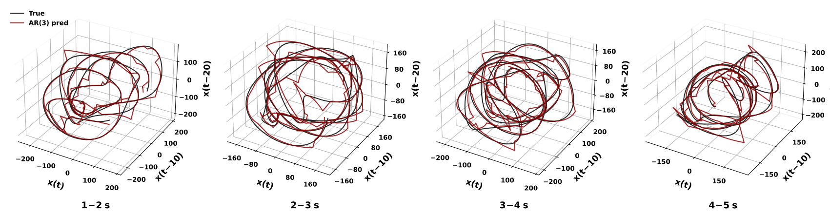
A long recording can superimpose several locally different geometries. Shorter views help distinguish a coherent local loop from the thicker cloud produced when phase relationships or amplitudes change over time. The next cell extracts 1-2, 2-3, 3-4, and 4-5 seconds and embeds the observed and reconstructed traces with the same delay in each panel.

The AR coefficients are reused; a separate model is not fitted to each displayed interval. Each predicted segment is matched to its observed segment’s mean and standard deviation before embedding. Compare loop opening, thickness, and relative trajectory shape, while remembering that absolute amplitude differences have been removed for display.

The full reconstruction includes both the initial training portion and later samples. These panels are views of that one reconstruction, not independently fitted or independent test trials.

Show code

Hide code

def plot_state_space_windows_comparison(xs, xs_pred, Fs, tau, embed_dim=3, 
                                         windows=[(1, 2), (2, 3), (3, 4), (4, 5)]):
    fig, axes = plt.subplots(1, 4, figsize=(len(windows)*4.5, 5), subplot_kw={'projection': '3d'})
    
    for ax, (t_start, t_end) in zip(axes, windows):
        idx_start = int(t_start * Fs)
        idx_end = int(t_end * Fs)
        
        # True signal
        segment_true = xs[idx_start:idx_end]
        X3_true = nfm.embedding.delay(np.asarray(segment_true, dtype=np.float32), dimension=embed_dim, tau_samples=tau)
        
        # Predicted signal (variance-matched)
        segment_pred = xs_pred[idx_start:idx_end]
        seg_pred_matched = segment_pred - np.mean(segment_pred)
        seg_pred_matched = seg_pred_matched * (np.std(segment_true) / (np.std(seg_pred_matched) + 1e-12))
        seg_pred_matched = seg_pred_matched + np.mean(segment_true)
        X3_pred = nfm.embedding.delay(np.asarray(seg_pred_matched, dtype=np.float32), dimension=embed_dim, tau_samples=tau)
        
        ax.plot(X3_true[:, 0], X3_true[:, 1], X3_true[:, 2], color='black', alpha=0.85, lw=1.5, label='True')
        ax.plot(X3_pred[:, 0], X3_pred[:, 1], X3_pred[:, 2], color='darkred', alpha=0.85, lw=1.5, label=f'AR({p_use}) pred')
        
        # Bold axis labels (LaTeX)
        ax.set_xlabel(r"$\mathbf{x(t)}$", labelpad=8, fontsize=13)
        ax.set_ylabel(f"$\\mathbf{{x(t\\!-\\!{tau})}}$", labelpad=8, fontsize=13)
        ax.set_zlabel(f"$\\mathbf{{x(t\\!-\\!{2*tau})}}$", labelpad=8, fontsize=13)
        
        # Limit tick count to avoid crowding (adapts to data range)
        from matplotlib.ticker import MaxNLocator
        ax.xaxis.set_major_locator(MaxNLocator(nbins=5))
        ax.yaxis.set_major_locator(MaxNLocator(nbins=5))
        ax.zaxis.set_major_locator(MaxNLocator(nbins=5))
        ax.tick_params(axis='both', pad=4, labelsize=10)
        
        # Bold tick labels
        for label in ax.xaxis.get_ticklabels() + ax.yaxis.get_ticklabels() + ax.zaxis.get_ticklabels():
            label.set_fontweight('bold')
        
        # Remove grey background panes
        ax.xaxis.pane.fill = False
        ax.yaxis.pane.fill = False
        ax.zaxis.pane.fill = False
        
        # Bold time-window annotation
        ax.text2D(0.5, -0.12, f"$\\mathbf{{{t_start}\\!-\\!{t_end} \\; s}}$",
                  transform=ax.transAxes, ha='center', fontsize=14, fontweight='bold')
    
    axes[0].legend(frameon=False, loc='upper left', fontsize=11,
                   prop={'weight': 'bold'})
    fig.subplots_adjust(left=0.02, right=0.98, bottom=0.12, top=0.95, wspace=0.15)
    plt.tight_layout(pad=2.5, w_pad=1.5)
    plt.savefig("4.pdf", bbox_inches='tight', dpi=300)
    plt.show()

# Build full prediction for visualization
full_pred = nfm.models.ARFit(w[0], w[1:]).forecast(xs, start_sample=p_use, n_samples=len(xs)-p_use, refresh_samples=REFRESH_EVERY)
xs_pred_full = np.concatenate([xs[:p_use], full_pred])

plot_state_space_windows_comparison(xs, xs_pred_full, Fs, tau)

/tmp/ipykernel_3766439/1059032341.py:51: UserWarning: Tight layout not applied. The left and right margins cannot be made large enough to accommodate all Axes decorations.
  plt.tight_layout(pad=2.5, w_pad=1.5)

10. Inspect Sensitivity to the Embedding Delay

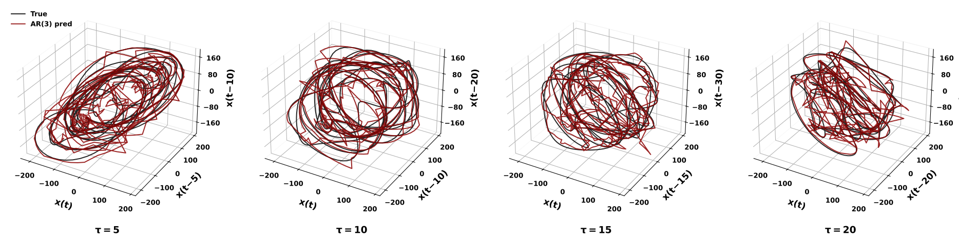
The next comparison holds the signal interval and fitted model fixed and changes only the coordinate delay. It uses 2-4 seconds, with \(\tau\) equal to 5, 10, 15, and 20 samples: 10, 20, 30, and 40 ms at 500 Hz.

When a delay is very small relative to the oscillatory timescale, adjacent coordinates are nearly identical, compressing the curve toward a diagonal. A larger delay can separate phases and reveal an opening. Still larger delays can alter the apparent shape, mix changing dynamics across a longer history, or align particular oscillations unfavorably. Larger is therefore not automatically better.

Each three-dimensional point spans \(2\tau\) samples of history, and the number of points decreases as the delay increases. Judge the displayed differences as changes of representation, not changes to the underlying recording or additional fitted models. A useful delay resolves the relevant temporal structure and remains interpretable across nearby choices and time windows; an attractive isolated view alone is not a topology estimate.

Show code

Hide code

def plot_state_space_tau_sweep(xs, xs_pred, Fs, t_start, t_end, taus=[5, 10, 15, 20], embed_dim=3):
    fig, axes = plt.subplots(1, 4, figsize=(20, 5), subplot_kw={'projection': '3d'})
    
    idx_start = int(t_start * Fs)
    idx_end = int(t_end * Fs)
    segment_true = xs[idx_start:idx_end]
    segment_pred = xs_pred[idx_start:idx_end]
    
    # Variance-match prediction
    seg_pred_matched = segment_pred - np.mean(segment_pred)
    seg_pred_matched = seg_pred_matched * (np.std(segment_true) / (np.std(seg_pred_matched) + 1e-12))
    seg_pred_matched = seg_pred_matched + np.mean(segment_true)
    
    for ax, tau_val in zip(axes, taus):
        X3_true = nfm.embedding.delay(np.asarray(segment_true, dtype=np.float32), dimension=embed_dim, tau_samples=tau_val)
        X3_pred = nfm.embedding.delay(np.asarray(seg_pred_matched, dtype=np.float32), dimension=embed_dim, tau_samples=tau_val)
        
        ax.plot(X3_true[:, 0], X3_true[:, 1], X3_true[:, 2], color='black', alpha=0.85, lw=1.5, label='True')
        ax.plot(X3_pred[:, 0], X3_pred[:, 1], X3_pred[:, 2], color='darkred', alpha=0.85, lw=1.5, label=f'AR({p_use}) pred')
        
        # Bold axis labels (LaTeX)
        ax.set_xlabel(r"$\mathbf{x(t)}$", labelpad=8, fontsize=13)
        ax.set_ylabel(f"$\\mathbf{{x(t\\!-\\!{tau_val})}}$", labelpad=8, fontsize=13)
        ax.set_zlabel(f"$\\mathbf{{x(t\\!-\\!{2*tau_val})}}$", labelpad=8, fontsize=13)
        
        # Limit tick count to avoid crowding
        from matplotlib.ticker import MaxNLocator
        ax.xaxis.set_major_locator(MaxNLocator(nbins=5))
        ax.yaxis.set_major_locator(MaxNLocator(nbins=5))
        ax.zaxis.set_major_locator(MaxNLocator(nbins=5))
        ax.tick_params(axis='both', pad=4, labelsize=10)
        
        # Bold tick labels
        for label in ax.xaxis.get_ticklabels() + ax.yaxis.get_ticklabels() + ax.zaxis.get_ticklabels():
            label.set_fontweight('bold')
        
        # Remove grey background panes
        ax.xaxis.pane.fill = False
        ax.yaxis.pane.fill = False
        ax.zaxis.pane.fill = False
        
        # Bold caption
        ax.text2D(0.5, -0.12, f"$\\mathbf{{\\tau = {tau_val}}}$",
                  transform=ax.transAxes, ha='center', fontsize=14, fontweight='bold')
    
    axes[0].legend(frameon=False, loc='upper left', fontsize=11,
                   prop={'weight': 'bold'})
    fig.subplots_adjust(left=0.02, right=0.98, bottom=0.12, top=0.95, wspace=0.15)
    plt.tight_layout(pad=2.5, w_pad=1.5)
    plt.savefig("5.pdf", bbox_inches='tight', dpi=300)
    plt.show()

# Use valid time window within 5 second signal
plot_state_space_tau_sweep(xs, xs_pred_full, Fs, t_start=2, t_end=4)

/tmp/ipykernel_3766439/2192212464.py:49: UserWarning: Tight layout not applied. The left and right margins cannot be made large enough to accommodate all Axes decorations.
  plt.tight_layout(pad=2.5, w_pad=1.5)

11. Reconstruct Individual Recording Channels

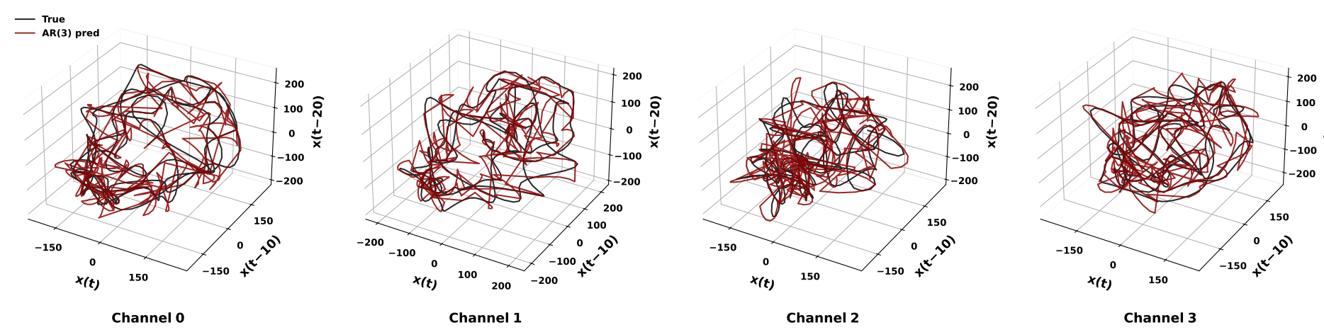
The final comparison repeats preprocessing and AR fitting separately for several channels. Each predictor uses only the history of its own channel. Signals are not averaged across electrodes, and a model trained on one channel is not used to predict another. This distinguishes a collection of univariate reconstructions from a multivariate model.

The four examples use channels 0-3, display intervals 5-6, 6-7, 8-9, and 10-11 seconds, and delays of 10 samples (20 ms). They require the full recording beyond the five-second snippet. The channel helper uses a 1-50 Hz bandpass, 500 Hz output, AR(3), 90% training, and five-sample history refreshes. In contrast, the initial single-channel example uses a 1-20 Hz bandpass, 10% training, and ten-sample refreshes. Both the data interval and some analysis settings therefore change in this panel.

Compare the observed and reconstructed trajectory within each panel first, then look for recurring geometry across panels. Each prediction is amplitude-matched to its corresponding observed interval. Since the displayed times can differ and neighboring electrodes can share activity, these panels are illustrative comparisons, not independent evidence of distinct sources or a cross-channel prediction benchmark.

Show code

Hide code

def sweep_channels_plot(raw_data, channels, time_windows, taus, fs_orig,
                        p=3, train_frac=0.9, refresh_every=5,
                        bandpass_low=1.0, bandpass_high=50.0, 
                        fband=(1, 80), env_lp_hz=3.0, embed_dim=3,
                        target_Fs=500):
    """
    Process multiple channels from mouse data and plot state space comparison.
    """
    n = len(channels)
    fig, axes = plt.subplots(1, n, figsize=(n*5, 5), subplot_kw={'projection': '3d'})
    if n == 1:
        axes = [axes]
    
    # Convert to (samples, channels) format
    LFP = raw_data.T
    
    for ax, chan, (t_start, t_end), tau_val in zip(axes, channels, time_windows, taus):
        # Create time window indices
        time_window = np.arange(int(t_end * fs_orig))
        
        # Process signal
        xs_ch, _, Fs_ch = process_signal(LFP, chan, fs_orig, time_window,
                                          bandpass_low=bandpass_low, bandpass_high=bandpass_high,
                                          fband=fband, env_lp_hz=env_lp_hz,
                                          target_Fs=target_Fs)
        
        # Fit AR model
        ar_res = fit_ar_model(xs_ch, Fs_ch, p=p, train_frac=train_frac, refresh_every=refresh_every)
        w_ch, xs_pred_ch = ar_res['w'], ar_res['xs_pred_full']
        
        # Extract window
        idx_start, idx_end = int(t_start * Fs_ch), int(t_end * Fs_ch)
        segment_true = xs_ch[idx_start:idx_end]
        segment_pred = xs_pred_ch[idx_start:idx_end]
        
        # Variance-match prediction
        seg_pred_matched = segment_pred - np.mean(segment_pred)
        seg_pred_matched = seg_pred_matched * (np.std(segment_true) / (np.std(seg_pred_matched) + 1e-12))
        seg_pred_matched = seg_pred_matched + np.mean(segment_true)
        
        # Embed
        X3_true = nfm.embedding.delay(np.asarray(segment_true, dtype=np.float32), dimension=embed_dim, tau_samples=tau_val)
        X3_pred = nfm.embedding.delay(np.asarray(seg_pred_matched, dtype=np.float32), dimension=embed_dim, tau_samples=tau_val)
        
        # Plot
        ax.plot(X3_true[:, 0], X3_true[:, 1], X3_true[:, 2], color='black', alpha=0.85, lw=1.5, label='True')
        ax.plot(X3_pred[:, 0], X3_pred[:, 1], X3_pred[:, 2], color='darkred', alpha=0.85, lw=1.5, label=f'AR({p}) pred')
        
        # Bold axis labels (LaTeX)
        ax.set_xlabel(r"$\mathbf{x(t)}$", labelpad=8, fontsize=13)
        ax.set_ylabel(f"$\\mathbf{{x(t\\!-\\!{tau_val})}}$", labelpad=8, fontsize=13)
        ax.set_zlabel(f"$\\mathbf{{x(t\\!-\\!{2*tau_val})}}$", labelpad=8, fontsize=13)
        
        # Limit tick count to avoid crowding
        from matplotlib.ticker import MaxNLocator
        ax.xaxis.set_major_locator(MaxNLocator(nbins=5))
        ax.yaxis.set_major_locator(MaxNLocator(nbins=5))
        ax.zaxis.set_major_locator(MaxNLocator(nbins=5))
        ax.tick_params(axis='both', pad=4, labelsize=10)
        
        # Bold tick labels
        for label in ax.xaxis.get_ticklabels() + ax.yaxis.get_ticklabels() + ax.zaxis.get_ticklabels():
            label.set_fontweight('bold')
        
        # Remove grey background panes
        ax.xaxis.pane.fill = False
        ax.yaxis.pane.fill = False
        ax.zaxis.pane.fill = False
        
        # Bold caption
        ax.text2D(0.5, -0.12, f"$\\mathbf{{Channel \\; {chan}}}$",
                  transform=ax.transAxes, ha='center', fontsize=14, fontweight='bold')
    
    axes[0].legend(frameon=False, loc='upper left', fontsize=11,
                   prop={'weight': 'bold'})
    fig.subplots_adjust(left=0.02, right=0.98, bottom=0.12, top=0.95, wspace=0.15)
    plt.tight_layout(pad=2.5, w_pad=1.5)
    plt.savefig("6.pdf", bbox_inches='tight', dpi=300)
    plt.show()

# Load full raw data for multi-channel sweep
raw_data_full = np.load(filename)
print(f"Full data shape: {raw_data_full.shape}")

# Sweep across channels (using valid channels and time windows)
sweep_channels_plot(
    raw_data_full, 
    channels=[0, 1, 2, 3],
    time_windows=[(5, 6), (6, 7), (8, 9), (10, 11)],
    taus=[10, 10, 10, 10],
    fs_orig=fs_original,
    target_Fs=500
)

Full data shape: (4, 10841760)

/tmp/ipykernel_3766439/806345731.py:77: UserWarning: Tight layout not applied. The left and right margins cannot be made large enough to accommodate all Axes decorations.
  plt.tight_layout(pad=2.5, w_pad=1.5)

12. What to Take from the Reconstruction

This example connects a 1-20 Hz processed waveform to a fitted AR(3) predictor and a three-dimensional delay trajectory. The waveform, residual ACF, scatter plot, and state-space views answer complementary questions:

• Waveform and scatter: does the model reproduce sample timing and amplitude under the stated history-refresh protocol?

• Residual ACF: what temporal structure remains in its errors?

• Delay geometry: does the amplitude-matched reconstruction follow the observed local trajectory, and how does that comparison depend on the window and delay?

• Channel views: does a similar reconstruction remain useful for other individual traces under their displayed settings?

Use these views together. A high correlation does not establish correct topology, and a visually open loop does not establish a particular number of independent modes. The preprocessing is offline, the AR coefficients are fixed within a fit, and observed-history refreshes constrain the reconstruction. These choices define what the figures demonstrate and how the example can be adapted.

To apply the workflow to another recording, begin with its actual sampling rate and array orientation, choose a physiologically relevant processing band, and keep model order, forecast horizon, and embedding delay distinct. Compare several time intervals rather than relying on a single visually appealing trajectory.

Continue with Intrinsic vs. Embedding Dimensionality for the connection between AR poles and oscillatory modes, or DeepLagField for learning time-varying coefficients and autoregressive order.