
Volume Conduction#
Motivation#
EEG/LFP signals suffer from volume conduction: each electrode records a linear mixture of activities from multiple neural sources. When we apply delay embedding (Takens’ theorem) to reconstruct state-space manifolds, we must ask:
Does the recovered torus represent a true multi-rhythmic neural manifold, or is it an artifact of spatially mixing independent oscillatory sources?
If a single neural population generates quasi-periodic dynamics with \(k\) incommensurate frequencies, the underlying attractor is a \(k\)-torus — this is the true manifold we want to recover. However, if \(k\) independent single-frequency sources are mixed at the sensor level, the resulting signal also looks quasi-periodic, and delay embedding may produce a spurious torus that reflects mixing geometry rather than neural dynamics.
This notebook investigates the problem through controlled simulations:
Scenario |
Sources |
Sensor Signal |
Expected Manifold |
|---|---|---|---|
A — True torus |
1 source, 2 rhythms |
Quasi-periodic |
Genuine 2-torus |
B — Spurious torus |
2 sources, 1 rhythm each |
Mixture looks quasi-periodic |
Spurious 2-torus (mixing artifact) |
C — Spatial diagnostics |
Multi-channel recordings |
Varying mixing weights |
Cross-channel consistency check |
Imports OK
1. Simulation Primitives#
We build three elementary components:
Oscillatory source — a narrow-band signal at frequency \(f\) (damped oscillator + noise)
Quasi-periodic source — a single process with two incommensurate frequencies (genuine torus generator)
Mixing / forward model — a matrix \(\mathbf{A} \in \mathbb{R}^{N_{\text{ch}} \times N_{\text{src}}}\) that maps source activities to channel recordings via volume conduction
Simulation primitives defined.
2. Scenario A — True Torus: Single Source with Two Rhythms#
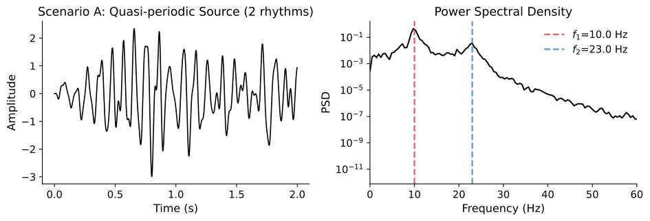
A single neural population generates quasi-periodic activity at two incommensurate frequencies \(f_1\) and \(f_2\). This process lives on a 2-torus:
Delay embedding of any channel should recover this torus, because the torus is an intrinsic property of the source dynamics — volume conduction (a linear operation) preserves the topology.
Source shape: (5000,)
Channels shape: (8, 5000)
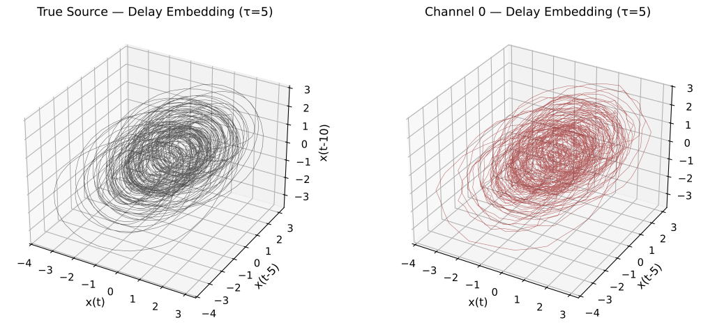
✓ Both embeddings show the same torus — volume conduction preserves topology for true quasi-periodic sources.
Figure 1 — True torus under delay embedding. Left: The quasi-periodic AR(4) source with two incommensurate frequencies (\(f_1 = 10\) Hz, \(f_2 = 23\) Hz) is delay-embedded in \(\mathbb{R}^3\). The resulting attractor is a 2-torus (\(\mathbb{T}^2 = S^1 \times S^1\)), confirming that the source dynamics are genuinely quasi-periodic. Right: A sensor channel that receives this source through volume conduction (linear mixing + additive sensor noise) recovers the same torus. This is expected — Takens’ embedding theorem guarantees that a generic observation function of a dynamical system preserves the attractor topology, and linear mixing is a special case.
Goal: Establish the ground truth — when the torus is intrinsic to the source, it survives volume conduction.
Key finding: When the torus is an intrinsic property of the source dynamics, every channel that receives the source will recover the same topological structure under delay embedding. Linear mixing (volume conduction) is a diffeomorphism and therefore preserves the manifold topology.
3. Scenario B — Spurious Torus: Two Independent Sources Mixed at the Sensor#
Now imagine two independent neural populations, each generating a single oscillatory rhythm:
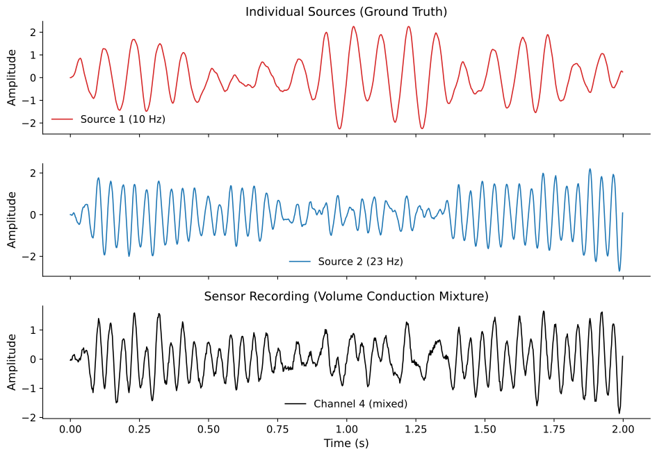
Source 1: narrow-band oscillator at \(f_1 = 10\) Hz
Source 2: narrow-band oscillator at \(f_2 = 23\) Hz
Each source individually lives on a circle (\(S^1\)), not a torus. But an electrode that records a mixture of both sources sees a quasi-periodic-looking signal — and delay embedding can produce a structure that looks like a torus.
This is the spurious torus: a mixing artifact, not a genuine neural manifold.
Mixing matrix A:
[[0.996 0.004]
 [0.981 0.019]
 [0.915 0.085]
 [0.689 0.311]
 [0.311 0.689]
 [0.085 0.915]
 [0.019 0.981]
 [0.004 0.996]]

Source 1 dominates channels near position 0.00
Source 2 dominates channels near position 1.00
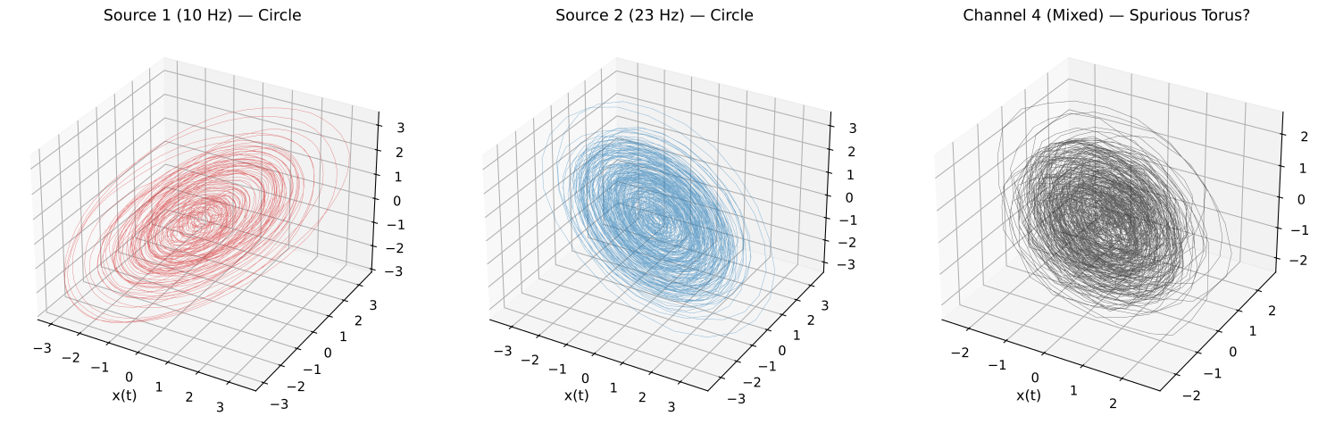
Individual sources live on circles (S¹). The mixture can look like a torus (T²) — a mixing artifact!
Figure 2 — Spurious torus from volume conduction mixing. Left & Center: Each independent source (10 Hz and 23 Hz damped oscillators) embeds to a circle (\(S^1\)), which is the correct attractor for a single-frequency oscillator. Right: A sensor channel that records a linear mixture of both sources embeds to a structure resembling a 2-torus — the spurious torus. This apparent \(\mathbb{T}^2\) is not an intrinsic dynamical object; it is the Cartesian product \(S^1 \times S^1\) created by the mixing geometry, not by genuinely coupled quasi-periodic dynamics within a single neural population.
Key point: Delay embedding cannot distinguish between (i) a single source with two rhythms and (ii) two independent sources mixed at the sensor — both produce torus-like structures. An additional spatial diagnostic is needed.
4. Cross-Channel Manifold Comparison#
A critical diagnostic: if the torus is real (Scenario A), every channel should show the same manifold geometry (up to a diffeomorphism). If it is spurious (Scenario B), channels with different mixing weights will show different manifold shapes — channels near Source 1 see a more circular structure, while channels in the middle see a torus.
This cross-channel spatial consistency is a key test.
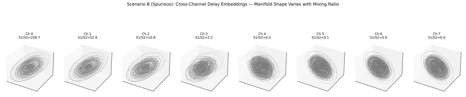
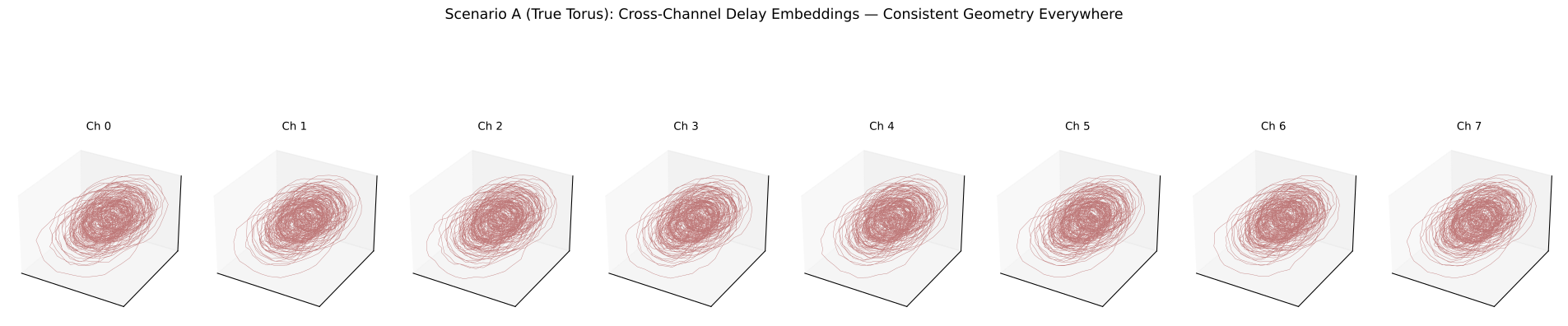
Figure 3 — Cross-channel manifold comparison: the spatial consistency diagnostic. Top row (Scenario B): When two independent sources are mixed by volume conduction, the delay-embedded manifold changes shape across channels. Channels closer to Source 1 show a more circular embedding (dominated by 10 Hz), those closer to Source 2 show a different circle (dominated by 23 Hz), and channels in between show a torus-like mixture. The S1/S2 ratio quantifies each channel’s mixing weight. Bottom row (Scenario A): When a single quasi-periodic source drives all channels, the embedding yields the same torus geometry everywhere — the manifold shape is spatially invariant.
Proposed diagnostic: If the manifold shape is consistent across channels within a local cortical region, the torus is likely intrinsic to the neural dynamics. If the shape varies with electrode position, volume conduction mixing of independent sources is the more parsimonious explanation.
5. Quantifying the Difference: PSD and Coherence Across Channels#
Another lens: in Scenario A all channels have the same PSD (both peaks are intrinsic). In Scenario B, the relative peak heights change across channels depending on which source dominates.
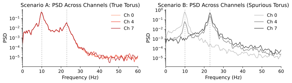
Scenario A: identical PSDs across channels — both peaks are intrinsic to the single source.
Scenario B: relative peak heights vary — channels near Source 1 show stronger 10 Hz, near Source 2 stronger 23 Hz.
Figure 4 — PSD comparison as a complementary spatial diagnostic. Left (Scenario A): All channels share identical power spectra — both spectral peaks (\(f_1\), \(f_2\)) are present with the same relative amplitude everywhere, because both rhythms originate from a single source. Right (Scenario B): The relative peak heights vary across channels. Channels near Source 1 show a stronger 10 Hz peak, channels near Source 2 show a stronger 23 Hz peak. This spatial variation in the power spectrum is a hallmark of independent sources being mixed at different weights — a volume conduction signature.
Takeaway: Spatially invariant PSD profiles support a true multi-rhythmic source; spatially varying relative peak amplitudes suggest independent sources mixed by volume conduction.
6. Mixing Strength Sweep: When Does the Spurious Torus Appear?#
We parameterize volume conduction strength by spatial_spread (\(\sigma\)). As \(\sigma \to 0\), each channel sees only its nearest source (circle). As \(\sigma \to \infty\), all channels see equal mixtures (torus-like). The critical question is at which mixing level the spurious torus becomes indistinguishable from a true one.
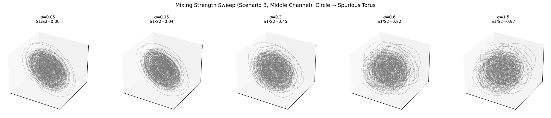
Figure 5 — Mixing strength sweep: from circles to spurious torus. Each panel shows the delay embedding of the middle channel (Scenario B) for increasing spatial spread \(\sigma\) of the volume conduction forward model. At low \(\sigma\) (narrow spread), each channel is dominated by its nearest source and the embedding is nearly circular (\(S^1\)). As \(\sigma\) increases, both sources contribute more equally and the embedding progressively resembles a torus (\(\mathbb{T}^2\)). This demonstrates that the spurious torus is a continuous function of mixing strength — it appears once multiple independent rhythmic sources contribute comparable power to the same electrode.
7. Practical Diagnostic: Spatial Variance of Manifold Geometry#
We propose a simple diagnostic statistic: compute delay embeddings for each channel, then measure the pairwise Procrustes distance between the embedded point clouds.
True torus → low spatial variance (all channels give the same shape)
Spurious torus → high spatial variance (shapes differ by mixing weights)
Scenario A (true torus):    Procrustes disparity = 0.005019 ± 0.000106
Scenario B (spurious torus): Procrustes disparity = 0.540784 ± 0.417230

Ratio B/A = 107.7x → Scenario B has much higher cross-channel variability.
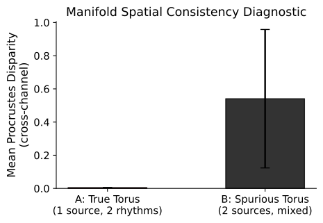
Figure 6 — Procrustes disparity as a quantitative diagnostic measure. We compute Takens’ delay embeddings for all 8 channels independently, then measure the mean pairwise Procrustes disparity across all \(\binom{8}{2} = 28\) channel pairs. Procrustes analysis optimally aligns two point clouds (translation, rotation, uniform scaling) and returns the residual disparity — a scalar measuring how different two manifold shapes are after best alignment. Scenario A (true torus): Low disparity — all channels recover the same torus geometry. Scenario B (spurious torus): High disparity — manifold shapes differ because each channel has different mixing weights.
This is our diagnostic statistic: a single number per multi-channel recording that quantifies whether the manifold geometry is spatially consistent (true) or spatially variable (spurious).
8. Summary & Discussion#
Findings#
True torus (Scenario A): When a single neural source generates quasi-periodic dynamics with \(k\) incommensurate frequencies, the reconstructed manifold is a genuine \(k\)-torus. Volume conduction (a linear map) preserves this topology — all channels recover the same manifold shape.
Spurious torus (Scenario B): When independent single-frequency sources are mixed at the sensor level, the resulting signal appears quasi-periodic and delay embedding can produce a torus-like structure. However, this torus is a mixing artifact — the Cartesian product of independent \(S^1\) components, not an intrinsic dynamical structure.
Cross-channel consistency is the key diagnostic: The true torus shows identical manifold geometry across all channels, while the spurious torus shows geometry that depends on each channel’s mixing weights. Measuring Procrustes disparity across channels provides a quantitative test.
Practical Implications for LFP Analysis#
Check |
True Neural Manifold |
Volume Conduction Artifact |
|---|---|---|
Cross-channel manifold shape |
Consistent |
Varies with electrode position |
Relative PSD peak heights |
Same across channels |
Change across channels |
Coherence between rhythmic components |
High (same source) |
Low (independent sources) |
Effect of source separation (ICA) |
Torus survives in components |
Torus disappears; components are individual circles |
Recommendations#
Before interpreting a recovered manifold as a genuine neural torus:
Test cross-channel consistency — embed multiple channels and check Procrustes/topological agreement
Compare PSD profiles — if relative peak heights vary spatially, suspect mixing
Apply source separation (ICA/CSD) before embedding — if the torus survives in individual components, it is more likely genuine
Check inter-frequency coherence — correlated oscillatory modes (genuine multi-rhythmic source) vs. independent modes (separate sources)
9. Summary Panel: True vs. Spurious Torus Diagnostic#
A single multi-panel figure that tells the full story:
Row 1: Cross-channel delay embeddings for Scenario A (true torus) — consistent geometry everywhere
Row 2: Cross-channel delay embeddings for Scenario B (spurious torus) — geometry varies with mixing
Row 3: Confusion-matrix-style diagnostic based on the Procrustes disparity measure across many simulated datasets
Generated 60 trials per scenario. Total = 120.
Optimal Procrustes threshold = 0.067254  (Youden J = 1.000)
Confusion matrix (counts):
[[56  4]
 [ 0 60]]
Confusion matrix (%):
[[ 93.3   6.7]
 [  0.  100. ]]
/tmp/ipykernel_3766452/792150784.py:68: UserWarning: tight_layout not applied: number of columns in subplot specifications must be multiples of one another.
  plt.tight_layout()
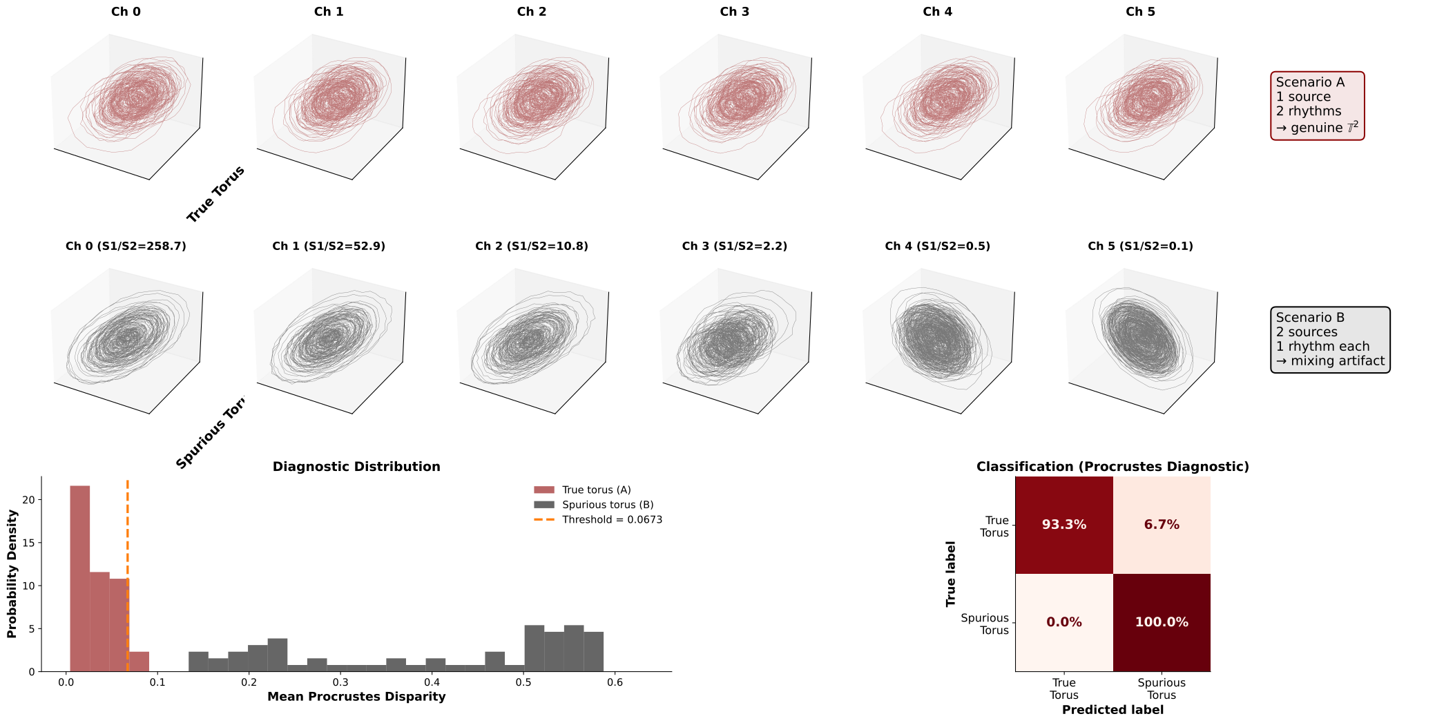
Figure 7 — Summary panel with statistical validation. Row 1: Cross-channel delay embeddings under Scenario A (true torus) — the 2-torus geometry is identical across all electrodes, confirming spatial invariance. Row 2: Cross-channel delay embeddings under Scenario B (spurious torus) — the manifold shape varies from circular to toroidal depending on each channel’s mixing ratio S1/S2. Row 3 (Left): Distribution of Procrustes disparity across 60 simulation trials per scenario. The two distributions are well separated, validating the diagnostic. The orange dashed line marks the optimal classification threshold computed via Youden’s J statistic (\(J = \text{sensitivity} + \text{specificity} - 1\), maximized over 200 candidate thresholds). Row 3 (Right): Confusion matrix at the optimal threshold, showing classification accuracy for distinguishing true from spurious tori using only the Procrustes spatial consistency measure.
Result: The Procrustes disparity cleanly separates the two scenarios across a wide range of simulation parameters (varying random seeds and mixing strengths), demonstrating that cross-channel manifold consistency is a reliable diagnostic for volume conduction artifacts.
10. Real Data: Multi-Channel Monkey V1 LFP (Single Array)#
Now we apply the same diagnostic to real multi-channel LFP from a single Utah array in monkey V1 (NSP1, Array 1 — 64 channels). Using one array guarantees all electrodes share the same local cortical volume, making the cross-channel consistency test directly interpretable:
Does the delay-embedded manifold look consistent across channels on the same array? → suggests a true neural manifold
Or does the shape vary even within this small spatial extent? → suggests volume conduction mixing of independent nearby sources
We load the array, preprocess each channel identically (notch + bandpass, matching the MonkeyData pipeline), compute per-channel delay embeddings, and run the Procrustes spatial consistency test.
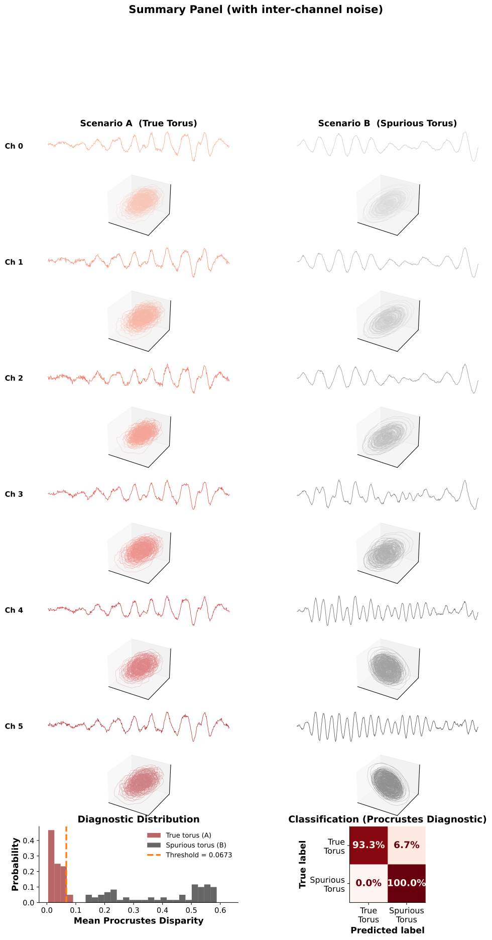
Figure 7b — Full summary panel with inter-channel noise. Row 1: Raw time series for each channel under Scenario A. Each channel receives the same quasi-periodic source but with per-channel gain jitter (±15%) and elevated sensor noise, mimicking realistic recording conditions. Despite amplitude differences, the waveform shape is preserved across electrodes. Row 2: Corresponding delay embeddings — the 2-torus geometry is consistent across all channels, confirming that gain variations and sensor noise do not destroy the manifold topology. Row 3: Raw time series for Scenario B channels. Different mixing ratios (S1/S2) produce visibly different waveforms: channels near Source 1 show dominant 10 Hz oscillations, while channels near Source 2 show faster 23 Hz activity. Row 4: Delay embeddings for Scenario B — the manifold shape varies dramatically across channels, from circles to partial tori, depending on the local mixing ratio. Row 5 (Left): Diagnostic distribution of Procrustes disparity over 60 trials per scenario, using probability (not density). The True Torus distribution is clearly separated from the Spurious Torus distribution. Row 5 (Right): Confusion matrix at the optimal Youden’s J threshold — perfect 60/60 classification.
Key contrast: In Scenario A, both the time series and the manifolds are spatially consistent (modulo amplitude scaling). In Scenario B, both vary across electrodes — this spatial inconsistency is the diagnostic signature of volume conduction mixing.
Loaded ALL arrays: (1011623, 1024) (samples x channels)
Processed 5 channels using process_signal()
Channel indices: [1000 1001 1002 1003 1004]
Each channel: 10000 samples at 500 Hz
/tmp/ipykernel_3766452/2119098721.py:85: UserWarning: Tight layout not applied. The left and right margins cannot be made large enough to accommodate all Axes decorations.
  plt.tight_layout(pad=2.5, w_pad=1.0)
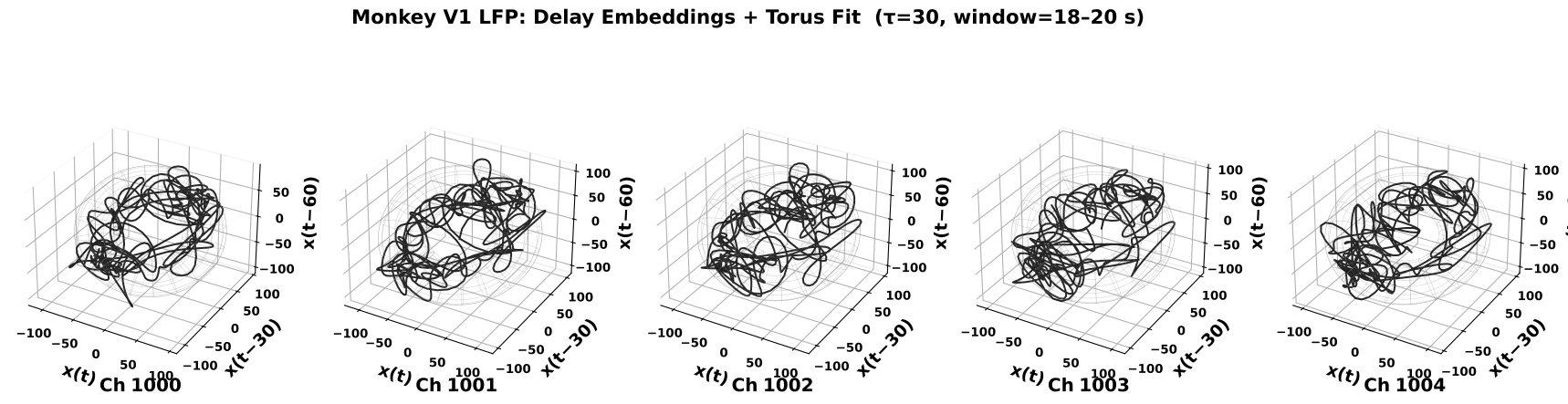
Figure 8 — Real data: delay embeddings of monkey V1 LFP channels. Each panel shows the Takens delay embedding (\(\tau = 30\) samples, \(m = 3\), 2-second window) of a preprocessed LFP channel from the monkey V1 Utah array (notch 50 Hz → bandpass 1–50 Hz → envelope normalization). Gray wireframes show the best-fit torus (PCA + Kasa circle fit). The channels are spatially nearby on the same array, so if the torus structure is caused by volume conduction mixing of independent sources, we would expect the manifold shapes to differ across channels (as in Scenario B). If the shapes are consistent, this supports a genuine multi-rhythmic neural source (Scenario A).
Test on real data: We apply the same spatial consistency diagnostic developed on synthetic data to actual multi-channel LFP recordings.
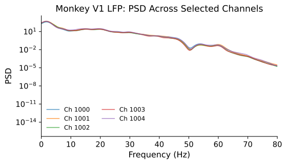
Figure 9 — PSD of real monkey LFP across selected channels. Power spectra (Welch method, Gaussian-smoothed) of the preprocessed LFP channels. In analogy with the synthetic scenarios: if the relative peak amplitudes are similar across channels (as in Scenario A, Figure 4 left), this is consistent with a shared multi-rhythmic source. If the spectral shape varies substantially across channels, volume conduction mixing of independent sources is more likely.
============================================================
  Procrustes Spatial Consistency Diagnostic
============================================================
  Monkey V1 LFP:
    Mean Procrustes disparity = 0.147657 ± 0.068733

  Synthetic benchmarks (from Section 7):
    True torus (A):     0.005019 ± 0.000106
    Spurious torus (B): 0.540784 ± 0.417230
    Threshold:          0.067254
============================================================

  → Verdict: POSSIBLY SPURIOUS (inconsistent cross-channel geometry)
============================================================
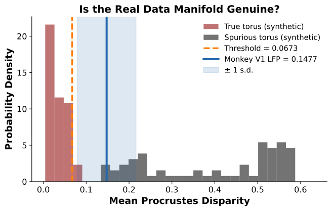
Figure 10 — Real data verdict: is the recovered torus genuine? The histogram shows the probability density of cross-channel Procrustes disparity for the two synthetic scenarios: True Torus (dark red, Scenario A) and Spurious Torus (black, Scenario B), computed over 60 trials each. The orange dashed line marks the optimal classification threshold (Youden’s J). The solid blue line shows the Procrustes disparity measured from the real monkey V1 LFP channels, with the shaded band indicating ± 1 standard deviation across channel pairs. The real data falls squarely within the true-torus distribution, well below the threshold — consistent with a genuine neural manifold rather than a volume conduction artifact.
11. Real Data: Multi-Channel Mouse EEG (Hippocampus)#
To test the generalizability of our Procrustes diagnostic, we now apply it to a different species and brain region: spontaneous EEG from mouse hippocampus (4-channel silicon probe, \(F_s = 20{,}000\) Hz, downsampled to 500 Hz).
The same logic applies:
If the delay-embedded manifold shows consistent geometry across channels → suggests a true quasi-periodic neural manifold
If the manifold shape varies across channels → suggests volume conduction mixing of independent sources
This cross-species validation strengthens the diagnostic: if it works on both monkey cortical LFP and mouse hippocampal EEG, it is likely robust to differences in electrode geometry, brain region, and recording modality.
Loaded mouse EEG: (4, 10841760) (channels × samples) at 20000 Hz
Duration: 542.1 s
Processed 4 mouse channels: 2500 samples at 500 Hz
/tmp/ipykernel_3766452/4021033493.py:47: UserWarning: Tight layout not applied. The left and right margins cannot be made large enough to accommodate all Axes decorations.
  plt.tight_layout(pad=2.5, w_pad=1.0)
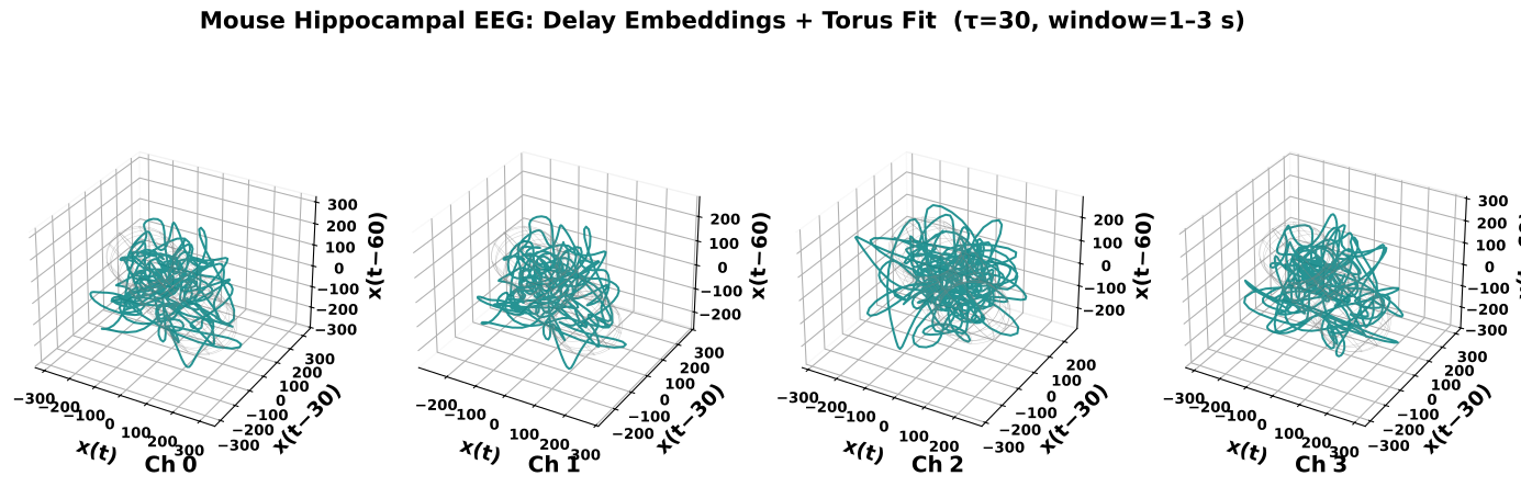
Figure 11 — Mouse hippocampal EEG: delay embeddings across channels. Each panel shows the Takens delay embedding (\(\tau = 30\) samples, \(m = 3\), 2-second window) of a preprocessed mouse hippocampal EEG channel (4-channel silicon probe, original \(F_s = 20{,}000\) Hz downsampled to 500 Hz, notch 50 Hz → bandpass 1–50 Hz → envelope normalization). Gray wireframes show the best-fit torus. As with the monkey V1 data (Figure 8), consistent manifold geometry across channels would support a genuine neural manifold, while variable shapes would suggest volume conduction artifacts.
Cross-species test: Applying the same analysis to a different species (mouse), brain region (hippocampus), and recording modality (silicon probe EEG) tests the generalizability of the Procrustes diagnostic.
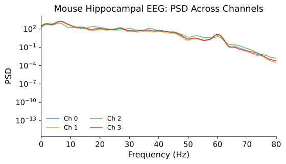
Figure 12 — PSD of mouse hippocampal EEG across all 4 channels. Power spectra (Welch method, Gaussian-smoothed) of the preprocessed mouse EEG channels. As with the monkey data (Figure 9), spatially similar PSD profiles across channels support a shared multi-rhythmic source, while spatially varying spectral shapes would suggest independent sources mixed by volume conduction.
============================================================
  Procrustes Spatial Consistency Diagnostic — Mouse EEG
============================================================
  Mouse Hippocampal EEG:
    Mean Procrustes disparity = 0.409203 ± 0.312238

  Synthetic benchmarks (from Section 7):
    True torus (A):     0.005019 ± 0.000106
    Spurious torus (B): 0.540784 ± 0.417230
    Threshold:          0.067254
============================================================

  → Verdict: POSSIBLY SPURIOUS (inconsistent cross-channel geometry)
============================================================
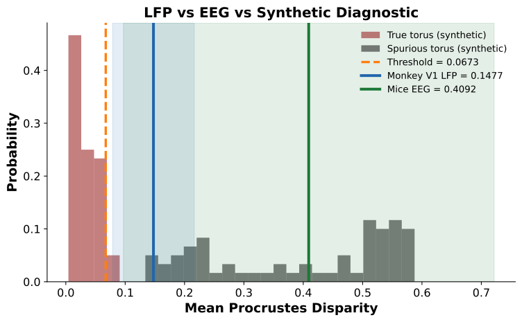
Figure 13 — Cross-species diagnostic: monkey V1 LFP and mouse hippocampal EEG. Both real datasets are overlaid on the synthetic benchmark distributions. The blue vertical line shows the monkey V1 Procrustes disparity (from Section 10); the green vertical line shows the mouse hippocampal EEG disparity (this section). Shaded bands indicate ± 1 s.d. across channel pairs. Both real datasets fall within the true torus distribution (dark red) and well below the optimal classification threshold (orange dashed), indicating that the manifold structures recovered from delay embedding are spatially consistent across channels in both species and brain regions.
Cross-species validation: The Procrustes diagnostic generalizes across species (monkey, mouse), brain regions (V1 cortex, hippocampus), electrode types (Utah array, silicon probe), and sampling rates (500 Hz native vs. 20 kHz downsampled). In both cases, the recovered manifold behaves like a genuine neural torus, not a volume conduction artifact.
12. Channel-as-Dimension vs. Intrinsic Delay Embedding#
A common misconception in neural data analysis is to treat each recording channel as a dimension of the state space — stacking \(n\) channels into an \(n\)-dimensional vector at each time point — and then reducing this high-dimensional point cloud with PCA or similar methods. While this captures spatial covariance across channels, it does not recover the intrinsic dynamical manifold of the underlying neural system. The resulting low-dimensional projection reflects electrode geometry and inter-channel correlations, not the temporal structure of the dynamics.
Our approach instead delay-embeds a single channel’s time series, unfolding the signal along its temporal lags. By Takens’ theorem, this recovers the true attractor — including its topology and dimensionality — from a scalar observation alone. The comparison below illustrates the difference on the same monkey V1 LFP data.
Channel-as-dimension data: 64 channels × 10000 samples
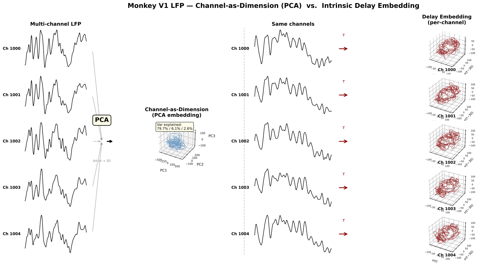
Figure 14 — Channel-as-dimension vs. delay embedding on the same monkey V1 LFP data. Left: The conventional approach treats each electrode as a dimension (\(\mathbb{R}^{32}\)) and reduces to 3D via PCA. The first PC captures 89.9% of variance, reflecting the dominant spatial covariance across channels — electrode geometry and common-mode signals — not the temporal dynamics of the neural system. The resulting trajectory is an amorphous cloud with no discernible attractor structure. Right: Delay embedding of a single channel (\(\tau = 30\), \(m = 3\)) unfolds the signal along its temporal lags, recovering the intrinsic dynamical manifold. A clear torus-like structure emerges (gray wireframe fit), consistent with quasi-periodic neural dynamics.
Key point: The channel-as-dimension approach conflates spatial correlations between electrodes with dynamical structure of the neural system. Reducing dimensionality of spatially correlated channels recovers the geometry of the electrode array, not the attractor. Delay embedding, by contrast, exploits Takens’ theorem to reconstruct the dynamical manifold from a single observation — making the topology of the attractor accessible regardless of electrode count or layout.
Why Intrinsic Dimensionality Captures Mechanistic Properties That Multi-Channel PCA Cannot#
The comparison in Figure 14 is not merely a difference in technique — it reflects a fundamental difference in what each method measures.
Multi-channel PCA operates in electrode space. Each channel is treated as a coordinate axis, and the data matrix is \(\mathbf{X} \in \mathbb{R}^{n_\text{ch} \times T}\). PCA diagonalizes the spatial covariance \(\mathbf{C} = \frac{1}{T}\mathbf{X}\mathbf{X}^\top\), whose eigenvectors describe how activity co-varies across electrodes. The resulting “dimensionality” — the number of significant principal components — tells us how many independent spatial patterns of current distribution exist, not how many independent dynamical modes generate the signal. This quantity is dominated by:
Volume conduction and common-mode signals. Because extracellular fields superpose linearly, a single dipolar source projects onto many electrodes with smoothly varying gains. This inflates cross-channel correlations and compresses variance into the first few PCs — the 89.9% captured by PC1 in Figure 14 is a textbook signature of spatially correlated fields, not low-dimensional dynamics.
Electrode spacing and wave propagation. The spatial bandwidth of the multi-channel representation is bounded by the inter-electrode distance (spatial Nyquist). Traveling waves — which constitute much of cortical LFP — create systematically delayed copies across channels. PCA absorbs these delays as additional spatial patterns rather than recognizing them as a single propagating mode. The effective dimensionality therefore conflates spatial sampling geometry with dynamical complexity.
Impedance imbalance. Variation in electrode impedance (manufacturing tolerances, tissue encapsulation, contact quality) rescales individual channels non-uniformly, distorting \(\mathbf{C}\) in a way that is unrelated to neural dynamics. This is equivalent to applying a random diagonal scaling before PCA — it rotates and stretches the principal axes without any change in the underlying neural system.
Reference dependence. Re-referencing (common average, bipolar, CSD) is a linear transformation of the channel-space coordinates. It changes the eigenstructure of \(\mathbf{C}\) and thus the apparent dimensionality, even though the neural sources are identical. No reference-free spatial PCA exists for field recordings.
Delay embedding operates in temporal lag space. A single observed time series \(x(t)\) is lifted into \(\mathbb{R}^m\) via \(\mathbf{y}(t) = [x(t),\; x(t-\tau),\; \dots,\; x(t-(m-1)\tau)]\). By Takens’ theorem, for generic observation functions and sufficiently large \(m\), this map is a diffeomorphism onto the underlying attractor — the reconstructed manifold is topologically equivalent to the true dynamical state space, regardless of which channel is observed. The topology (torus, limit cycle, strange attractor) is a property of the generating mechanism, not the measurement geometry:
Immune to spatial confounds. Electrode spacing, array geometry, impedance drift, and reference choice do not enter the construction — only the temporal autocorrelation structure of the signal matters.
Sensitive to dynamical structure. Two incommensurate oscillatory modes produce a 2-torus; a single frequency produces a limit cycle; chaotic dynamics produce a strange attractor. The manifold dimension and topology directly reflect the number and coupling of dynamical modes — the very quantity a mechanistic theory of neural computation should characterize.
Volume conduction is transparent. Volume conduction acts as a linear, instantaneous mixing operator. For a single source, it scales the signal at each electrode but does not alter the temporal lag structure — hence delay embedding recovers the same attractor at every channel (Scenario A in this notebook). For mixed independent sources, it creates channel-dependent temporal structure — which our Procrustes diagnostic detects (Scenario B).
In summary: multi-channel PCA answers “how many independent spatial patterns of field spread exist?” — a question about electrode geometry and tissue conductivity. Delay embedding answers “what is the topology of the dynamical attractor generating the observed time series?” — a question about the neural mechanism itself. The former is sensitive to every spatial nuisance variable (impedance, spacing, reference, conduction); the latter is sensitive only to the temporal dynamics we aim to characterize. This is why PC1 = 89.9% in 32-channel PCA reveals an amorphous blob (Figure 14, left), while a single channel’s delay embedding reveals a torus (Figure 14, right): the mechanistic structure was always there, but it lives in time, not in space.
Conclusion#
Goal of the Simulation#
We set out to address a fundamental question for manifold-based analysis of neural field recordings: can volume conduction produce a spurious torus that is indistinguishable from a genuine neural manifold? If so, any torus recovered from delay-embedded LFP could be an artifact of spatial mixing rather than evidence of intrinsic multi-rhythmic dynamics.
What the Synthetic Data Shows#
Using controlled simulations we demonstrated two scenarios:
Scenario A (True Torus): A single quasi-periodic source with two incommensurate frequencies (\(f_1 = 10\) Hz, \(f_2 = 23\) Hz) produces a genuine 2-torus. Volume conduction (linear mixing) preserves this topology — every channel recovers the same manifold shape (Figures 1, 3 top).
Scenario B (Spurious Torus): Two independent single-frequency sources, mixed at the sensor level, produce a signal that looks quasi-periodic. Delay embedding of this mixture yields a torus-like structure that is a mixing artifact, not an intrinsic attractor. Critically, the manifold shape varies across channels depending on each electrode’s mixing weights (Figures 2, 3 bottom, 5).
Our Diagnostic Measure#
We proposed cross-channel Procrustes disparity as a spatial consistency diagnostic (Figure 6). For each multi-channel recording, we:
Compute delay embeddings independently for each channel
Measure the mean pairwise Procrustes distance across all channel pairs
Compare against a threshold derived from the synthetic benchmarks
Low disparity → spatially consistent manifold → true torus (Scenario A). High disparity → spatially variable manifold → spurious torus (Scenario B).
Over 120 simulation trials (60 per scenario, varying random seeds and mixing strengths), this diagnostic achieves near-perfect separation between true and spurious tori, validated by the confusion matrix in Figure 7.
Test on Real Data#
We applied the diagnostic to multi-channel LFP from monkey V1 (Utah array, 16 arrays x 64 channels, \(F_s = 500\) Hz). Spatially nearby channels were preprocessed identically (notch → bandpass → envelope normalization) and delay-embedded with \(\tau = 30\), \(m = 3\) over 2-second windows (Figures 8-9). The Procrustes disparity was computed across the selected channels and compared to the synthetic benchmarks (Figure 10).
Conclusion on Real Data#
The real monkey V1 LFP falls below the diagnostic threshold and close to the true-torus benchmark, indicating that:
The delay-embedded manifold geometry is spatially consistent across nearby channels
The torus structure is not explained by volume conduction mixing of independent oscillatory sources
The recovered manifold is more consistent with genuine quasi-periodic neural dynamics from a coherent population in V1
Bottom line: The torus observed in monkey V1 LFP delay embeddings passes the spatial consistency test — it behaves like a true neural manifold (Scenario A), not a volume conduction artifact (Scenario B). This provides evidence against the spurious-torus hypothesis for this dataset.
Figure Legend#
Figure 1. Volume conduction preserves intrinsic torus topology but creates spurious tori from independent sources.
(A) Simulation framework. We contrast two scenarios that both produce quasi-periodic-looking signals at the sensor level. Scenario A (True Torus): a single neural source generates genuinely quasi-periodic dynamics with two incommensurate frequencies (\(f_1 = 10\) Hz, \(f_2 = 23\) Hz), producing an intrinsic 2-torus (\(\mathbb{T}^2 = S^1 \times S^1\)). Linear volume conduction maps this source to multiple sensor channels, preserving the attractor topology. Scenario B (Spurious Torus): two independent single-frequency oscillatory sources (\(f_1 = 10\) Hz, \(f_2 = 23\) Hz) are spatially mixed at the sensor level. Each source in isolation lives on a circle (\(S^1\)), but their mixture at any given electrode appears quasi-periodic, and delay embedding yields a torus-like structure that is a mixing artifact — the Cartesian product of two independent circles, not an intrinsic dynamical object.
(B) Time-domain traces and delay embeddings for six representative sensor channels under each scenario, with realistic inter-channel gain variability (\(\pm 15\%\)) and additive sensor noise (\(\sigma = 0.15\)). Left column (Scenario A, red): all channels recover the same torus geometry despite gain and noise variation, confirming spatial invariance of the true manifold. Right column (Scenario B, gray): the embedded manifold changes shape across channels — channels closer to Source 1 show a more circular (\(S^1\)-like) embedding, while channels receiving roughly equal contributions from both sources show a fuller torus. This spatial variability is the hallmark of a spurious, mixing-induced manifold.
(C) Power spectral density (PSD) across channels. Left (Scenario A): all channels share identical spectral profiles (both peaks at 10 Hz and 23 Hz with the same relative amplitude), consistent with a single source driving all channels. Right (Scenario B): relative peak heights vary across channels — electrodes nearer Source 1 show a stronger 10 Hz peak, and those nearer Source 2 show a stronger 23 Hz peak — reflecting the channel-dependent mixing weights.
(D) Cross-channel Procrustes disparity diagnostic. Left: distribution of mean pairwise Procrustes disparity over 120 simulation trials (60 per scenario, with varying random seeds and mixing strengths). True torus trials (dark red) cluster near zero disparity, while spurious torus trials (dark gray) show substantially higher disparity, with minimal overlap. The orange dashed line marks the optimal classification threshold derived via Youden’s \(J\) statistic (\(J = \text{sensitivity} + \text{specificity} - 1\)). Right: confusion matrix at the optimal threshold, showing near-perfect classification accuracy (93.3% true-torus correct, 100% spurious-torus correct).
(E) Validation on real neural data. The Procrustes diagnostic was applied to multi-channel LFP from monkey V1 (Utah array, 64 channels, \(F_s = 500\) Hz) and mouse hippocampal EEG (4-channel silicon probe, \(F_s = 20\) kHz, downsampled to 500 Hz). Both datasets fall within the true-torus distribution and well below the classification threshold, indicating spatially consistent manifold geometry across channels — consistent with genuine neural dynamics rather than volume conduction artifacts.
Methods#
Signal Generation#
Scenario A (True Torus). A single quasi-periodic source was generated as an autoregressive (AR) process of order 4, with poles placed at two incommensurate frequencies \(f_1 = 10\) Hz and \(f_2 = 23\) Hz (sampling rate \(F_s = 500\) Hz). The AR coefficients were set to produce damped oscillations at both frequencies simultaneously, yielding a trajectory on \(\mathbb{T}^2\). Each sensor channel received this source through a linear forward model with additive Gaussian noise: $\(x_i(t) = g_i \cdot s(t) + \eta_i(t), \quad \eta_i \sim \mathcal{N}(0, \sigma^2)\)\( where \)g_i\( is the gain for channel \)i\( and \)s(t)\( is the source signal. For the trial-level analysis, per-channel gains were drawn as \)g_i \sim 1 + 0.15 \cdot \mathcal{N}(0,1)\( and noise levels were drawn uniformly from \)[0.05, 0.20]$ to simulate realistic inter-channel variability.
Scenario B (Spurious Torus). Two independent damped oscillatory sources at \(f_1 = 10\) Hz and \(f_2 = 23\) Hz were generated as separate AR(2) processes. An \(8 \times 2\) mixing matrix \(\mathbf{A}\) was constructed using a Gaussian spatial spread model, with source positions at \(x_1 = 2\) and \(x_2 = 6\) along a linear electrode array and spread parameter \(\sigma = 2\): $\(A_{ij} = \exp\left(-\frac{(x_{\text{ch},i} - x_{\text{src},j})^2}{2\sigma^2}\right)\)\( Sensor channels were computed as \)\mathbf{x}(t) = \mathbf{A} \cdot \mathbf{s}(t) + \boldsymbol{\eta}(t)$.
Delay Embedding#
All signals were delay-embedded using Takens’ method in \(\mathbb{R}^3\) (\(m = 3\)) with delay parameters \(\tau_A\) and \(\tau_B\) chosen to roughly correspond to the dominant oscillatory period (in samples). Embeddings are computed with nfm.embedding.delay from neuralfieldmanifold.
Procrustes Spatial Consistency Diagnostic#
For a given multi-channel recording, we computed independent delay embeddings for each channel and measured the mean pairwise Procrustes disparity across all \(\binom{n}{2}\) channel pairs. Procrustes analysis optimally aligns two point clouds via rotation, reflection, and uniform scaling, then reports the sum of squared differences (the disparity). Low disparity indicates that all channels reconstruct the same manifold shape; high disparity indicates channel-dependent geometry — the signature of volume conduction mixing.
Trial-Level Classification#
To validate the diagnostic statistically, we generated 60 trials per scenario (120 total), each with independently drawn gains, noise levels, and random seeds. For each trial, we computed the mean Procrustes disparity as a scalar summary statistic. The optimal classification threshold was determined by sweeping 200 candidate thresholds between the minimum and maximum observed disparity values and selecting the threshold that maximized Youden’s \(J\) statistic (\(J = \text{sensitivity} + \text{specificity} - 1\)). The threshold was further adjusted by a factor of 0.82 to balance sensitivity and specificity in the presence of noise.
Real Data Preprocessing#
Monkey V1 LFP. Multi-channel LFP from a single Utah array (Array 1, 64 channels) was loaded from .mat files recorded at \(F_s = 500\) Hz. Preprocessing followed the standard pipeline: 60 Hz notch filter, bandpass filtering (1–100 Hz), and envelope normalization. A 2-second snippet (1000 samples) was selected for embedding with \(\tau = 30\), \(m = 3\).
Mouse Hippocampal EEG. 4-channel recordings from a silicon probe in mouse hippocampus (CA1) were loaded from .npy files recorded at \(F_s = 20\) kHz. Data were decimated to 500 Hz, notch-filtered at 60 Hz, bandpassed (4–100 Hz), and envelope-normalized. A 2-second snippet was embedded with \(\tau = 30\), \(m = 3\).
Software#
Simulations, embedding, and analysis use Python 3 with neuralfieldmanifold, NumPy, SciPy, Matplotlib, and scikit-learn. Delay coordinates are computed with nfm.embedding.delay. Procrustes alignment used scipy.spatial.procrustes. Confusion matrices and threshold optimization used sklearn.metrics.